pylbm is an all-in-one package for numerical simulations using Lattice Boltzmann solvers.
pylbm is licensed under the BSD license, enabling reuse with few restrictions.
pylbm can be a simple way to make numerical simulations by using the Lattice Boltzmann method.
To install pylbm, you have several ways. You can install it using conda
conda install pylbm -c pylbm -c conda-forge
or using the last version on Pypi
pip install pylbm
You can also clone the project
git clone https://github.com/pylbm/pylbm
and then use the command
python setup.py install
or if you don’t have root privileges
python setup.py install --user
Once the package is installed you just have to understand how build a dictionary that will be understood by pylbm to perform the simulation. The dictionary should contain all the needed informations as
the geometry (see here for documentation)
the scheme (see here for documentation)
the boundary conditions (see here for documentation)
another informations like the space step, the scheme velocity, the generator of the functions…
To understand how to use pylbm, you have a lot of Python notebooks in the tutorial.
With pylbm, the numerical simulations can be performed in a domain
with a complex geometry. This geometry is construct without considering a
particular mesh but only with geometrical objects.
All the geometrical informations are defined through a dictionary and
put into an object of the class Geometry.
First, the domain is put into a box: a segment in 1D, a rectangle in 2D, and a rectangular parallelepipoid in 3D.
Then, the domain is modified by adding or deleting some elementary shapes. In 2D, the elementary shapes are
From version 0.2, the geometrical elements are implemented in 3D. The elementary shapes are
Several examples of geometries can be found in demo/examples/geometry/
d = {'box':{'x': [0, 1], 'label': [0, 1]}}
g = pylbm.Geometry(d)
g.visualize(viewlabel = True)
# Authors:
#     Loic Gouarin <loic.gouarin@math.u-psud.fr>
#     Benjamin Graille <benjamin.graille@math.u-psud.fr>
#
# License: BSD 3 clause

"""
Example of a 1D geometry: the segment [0,1]
"""
import pylbm
d = {'box':{'x': [0, 1], 'label': [0, 1]}}
g = pylbm.Geometry(d)
g.visualize(viewlabel = True)
(Source code, png, pdf)

The segment \([0,1]\) is created by the dictionary with the key box.
We then add the labels 0 and 1 on the edges with the key label.
The result is then visualized with the labels by using the method
visualize.
If no labels are given in the dictionary, the default value is -1.
d = {'box':{'x': [0, 1], 'y': [0, 1]}}
g = pylbm.Geometry(d)
g.visualize()
# Authors:
#     Loic Gouarin <loic.gouarin@math.u-psud.fr>
#     Benjamin Graille <benjamin.graille@math.u-psud.fr>
#
# License: BSD 3 clause

"""
Example of a 2D geometry: the square [0,1]x[0,1]
"""
import pylbm
d = {'box':{'x': [0, 1], 'y': [0, 1]}}
g = pylbm.Geometry(d)
g.visualize()
(Source code, png, pdf)

The square \([0,1]^2\) is created by the dictionary with the key box.
The result is then visualized by using the method
visualize.
We then add the labels on each edge of the square through a list of integers with the conventions:
|
|
d = {'box':{'x': [0, 1], 'y': [0, 1], 'label':[0, 1, 2, 3]}}
g = pylbm.Geometry(d)
g.visualize(viewlabel = True)
# Authors:
#     Loic Gouarin <loic.gouarin@math.u-psud.fr>
#     Benjamin Graille <benjamin.graille@math.u-psud.fr>
#
# License: BSD 3 clause

"""
Example of a 2D geometry: the square [0,1]x[0,1] with labels
"""
import pylbm
d = {'box':{'x': [0, 1], 'y': [0, 1], 'label':[0, 1, 2, 3]}}
g = pylbm.Geometry(d)
g.visualize(viewlabel = True)
(Source code, png, pdf)

If all the labels have the same value, a shorter solution is to give only the integer value of the label instead of the list. If no labels are given in the dictionary, the default value is -1.
The unit square \([0,1]^2\) can be holed with a circle (script 1) or with a triangular or with a parallelogram (script 3)
In the first example,
a solid disc lies in the fluid domain defined by
a circle
with a center of (0.5, 0.5) and a radius of 0.125
d = {'box':{'x': [0, 1], 'y': [0, 1], 'label':0},
     'elements':[pylbm.Circle((.5, .5), .125, label = 1)],
}
g = pylbm.Geometry(d)
g.visualize(viewlabel=True)
# Authors:
#     Loic Gouarin <loic.gouarin@math.u-psud.fr>
#     Benjamin Graille <benjamin.graille@math.u-psud.fr>
#
# License: BSD 3 clause

"""
Example of a 2D geometry: the square [0,1]x[0,1] with a circular hole
"""
import pylbm
d = {'box':{'x': [0, 1], 'y': [0, 1], 'label':0},
     'elements':[pylbm.Circle((.5, .5), .125, label = 1)],
}
g = pylbm.Geometry(d)
g.visualize(viewlabel=True)
(Source code, png, pdf)

The dictionary of the geometry then contains an additional key elements
that is a list of elements.
In this example, the circle is labelized by 1 while the edges of the square by 0.
The element can be also a triangle
d = {'box':{'x': [0, 1], 'y': [0, 1], 'label':0},
      'elements':[pylbm.Triangle((0.,0.), (0.,.5), (.5, 0.), label = 1)],
}
g = pylbm.Geometry(d)
g.visualize(viewlabel=True)
# Authors:
#     Loic Gouarin <loic.gouarin@math.u-psud.fr>
#     Benjamin Graille <benjamin.graille@math.u-psud.fr>
#
# License: BSD 3 clause

"""
Example of a 2D geometry: the square [0,1]x[0,1] with a triangular hole
"""
import pylbm
d = {'box':{'x': [0, 1], 'y': [0, 1], 'label':0},
      'elements':[pylbm.Triangle((0.,0.), (0.,.5), (.5, 0.), label = 1)],
}
g = pylbm.Geometry(d)
g.visualize(viewlabel=True)
(Source code, png, pdf)

or a parallelogram
d = {'box':{'x': [0, 3], 'y': [0, 1], 'label':[1, 2, 0, 0]},
     'elements':[pylbm.Parallelogram((0.,0.), (.5,0.), (0., .5), label = 0)],
}
g = pylbm.Geometry(d)
g.visualize()
# Authors:
#     Loic Gouarin <loic.gouarin@math.u-psud.fr>
#     Benjamin Graille <benjamin.graille@math.u-psud.fr>
#
# License: BSD 3 clause

"""
Example of a 2D geometry: the square [0,1]x[0,1] with a step
"""
import pylbm
d = {'box':{'x': [0, 3], 'y': [0, 1], 'label':[1, 2, 0, 0]},
     'elements':[pylbm.Parallelogram((0.,0.), (.5,0.), (0., .5), label = 0)],
}
g = pylbm.Geometry(d)
g.visualize()
(Source code, png, pdf)

A complex geometry can be build by using a list of elements. In this example,
the box is fixed to the unit square \([0,1]^2\). A square hole is added with the
argument isfluid=False. A strip and a circle are then added with the argument
isfluid=True. Finally, a square hole is put. The value of elements
contains the list of all the previous elements. Note that the order of
the elements in the list is relevant.
square = pylbm.Parallelogram((.1, .1), (.8, 0), (0, .8), isfluid=False)
strip = pylbm.Parallelogram((0, .4), (1, 0), (0, .2), isfluid=True)
circle = pylbm.Circle((.5, .5), .25, isfluid=True)
inner_square = pylbm.Parallelogram((.4, .5), (.1, .1), (.1, -.1), isfluid=False)
d = {'box':{'x': [0, 1], 'y': [0, 1], 'label':0},
     'elements':[square, strip, circle, inner_square],
}
g = pylbm.Geometry(d)
g.visualize()
Once the geometry is built, it can be modified by adding or deleting other elements. For instance, the four corners of the cavity can be rounded in this way.
g.add_elem(pylbm.Parallelogram((0.1, 0.9), (0.05, 0), (0, -0.05), isfluid=True))
g.add_elem(pylbm.Circle((0.15, 0.85), 0.05, isfluid=False))
g.add_elem(pylbm.Parallelogram((0.1, 0.1), (0.05, 0), (0, 0.05), isfluid=True))
g.add_elem(pylbm.Circle((0.15, 0.15), 0.05, isfluid=False))
g.add_elem(pylbm.Parallelogram((0.9, 0.9), (-0.05, 0), (0, -0.05), isfluid=True))
g.add_elem(pylbm.Circle((0.85, 0.85), 0.05, isfluid=False))
g.add_elem(pylbm.Parallelogram((0.9, 0.1), (-0.05, 0), (0, 0.05), isfluid=True))
g.add_elem(pylbm.Circle((0.85, 0.15), 0.05, isfluid=False))
g.visualize()
# Authors:
#     Loic Gouarin <loic.gouarin@math.u-psud.fr>
#     Benjamin Graille <benjamin.graille@math.u-psud.fr>
#
# License: BSD 3 clause

"""
Example of a complex geometry in 2D
"""
import pylbm
square = pylbm.Parallelogram((.1, .1), (.8, 0), (0, .8), isfluid=False)
strip = pylbm.Parallelogram((0, .4), (1, 0), (0, .2), isfluid=True)
circle = pylbm.Circle((.5, .5), .25, isfluid=True)
inner_square = pylbm.Parallelogram((.4, .5), (.1, .1), (.1, -.1), isfluid=False)
d = {'box':{'x': [0, 1], 'y': [0, 1], 'label':0},
     'elements':[square, strip, circle, inner_square],
}
g = pylbm.Geometry(d)
g.visualize()
# rounded inner angles
g.add_elem(pylbm.Parallelogram((0.1, 0.9), (0.05, 0), (0, -0.05), isfluid=True))
g.add_elem(pylbm.Circle((0.15, 0.85), 0.05, isfluid=False))
g.add_elem(pylbm.Parallelogram((0.1, 0.1), (0.05, 0), (0, 0.05), isfluid=True))
g.add_elem(pylbm.Circle((0.15, 0.15), 0.05, isfluid=False))
g.add_elem(pylbm.Parallelogram((0.9, 0.9), (-0.05, 0), (0, -0.05), isfluid=True))
g.add_elem(pylbm.Circle((0.85, 0.85), 0.05, isfluid=False))
g.add_elem(pylbm.Parallelogram((0.9, 0.1), (-0.05, 0), (0, 0.05), isfluid=True))
g.add_elem(pylbm.Circle((0.85, 0.15), 0.05, isfluid=False))
g.visualize()
d = {'box':{'x': [0, 1], 'y': [0, 1], 'z':[0, 1], 'label':list(range(6))}}
g = pylbm.Geometry(d)
g.visualize(viewlabel=True)
# Authors:
#     Loic Gouarin <loic.gouarin@math.u-psud.fr>
#     Benjamin Graille <benjamin.graille@math.u-psud.fr>
#
# License: BSD 3 clause

"""
Example of a 3D geometry: the cube [0,1]x[0,1]x[0,1]
"""
from six.moves import range
import pylbm
d = {'box':{'x': [0, 1], 'y': [0, 1], 'z':[0, 1], 'label':list(range(6))}}
g = pylbm.Geometry(d)
g.visualize(viewlabel=True)
The cube \([0,1]^3\) is created by the dictionary with the key box.
The result is then visualized by using the method
visualize.
We then add the labels on each edge of the square through a list of integers with the conventions:
|
|
If all the labels have the same value, a shorter solution is to give only the integer value of the label instead of the list. If no labels are given in the dictionary, the default value is -1.
d = {
    'box':{'x': [0, 1], 'y': [0, 1], 'z':[0, 1], 'label':0},
    'elements':[pylbm.Sphere((.5,.5,.5), .25, label=1)],
}
g = pylbm.Geometry(d)
g.visualize(viewlabel=True)
# Authors:
#     Loic Gouarin <loic.gouarin@math.u-psud.fr>
#     Benjamin Graille <benjamin.graille@math.u-psud.fr>
#
# License: BSD 3 clause

"""
Example of a 3D geometry: the cube [0,1]x[0,1]x[0,1]
"""
import pylbm
d = {
    'box':{'x': [0, 1], 'y': [0, 1], 'z':[0, 1], 'label':0},
    'elements':[pylbm.Sphere((.5,.5,.5), .25, label=1)],
}
g = pylbm.Geometry(d)
g.visualize(viewlabel=True)
The cube \([0,1]^3\) and the spherical hole are created
by the dictionary with the keys box and elements.
The result is then visualized by using the method
visualize.
With pylbm, the numerical simulations can be performed in a domain
with a complex geometry.
The creation of the geometry from a dictionary is explained here.
All the informations needed to build the domain are defined through a dictionary
and put in a object of the class Domain.
The domain is built from three types of informations:
a geometry (class Geometry),
a stencil (class Stencil),
a space step (a float for the grid step of the simulation).
The domain is a uniform cartesian discretization of the geometry with a grid step
\(dx\). The whole box is discretized even if some elements are added to reduce
the domain of the computation.
The stencil is necessary in order to know the maximal velocity in each direction
so that the corresponding number of phantom cells are added at the borders of
the domain (for the treatment of the boundary conditions).
The user can get the coordinates of the points in the domain by the fields
x, y, and z.
By convention, if the spatial dimension is one, y=z=None; and if it is two, z=None.
Several examples of domains can be found in demo/examples/domain/
dico = {
    'box':{'x': [0, 1], 'label':0},
    'space_step':0.1,
    'schemes':[{'velocities':list(range(3))}],
}
dom = pylbm.Domain(dico)
dom.visualize()
# Authors:
#     Loic Gouarin <loic.gouarin@math.u-psud.fr>
#     Benjamin Graille <benjamin.graille@math.u-psud.fr>
#
# License: BSD 3 clause

"""
Example of a segment in 1D with a D1Q3
"""
from six.moves import range
import pylbm
dico = {
    'box':{'x': [0, 1], 'label':0},
    'space_step':0.1,
    'schemes':[{'velocities':list(range(3))}],
}
dom = pylbm.Domain(dico)
dom.visualize()
(Source code, png, pdf)

The segment \([0,1]\) is created by the dictionary with the key box.
The stencil is composed by the velocity \(v_0=0\), \(v_1=1\), and
\(v_2=-1\). One phantom cell is then added at the left and at the right of
the domain.
The space step \(dx\) is taken to \(0.1\) to allow the visualization.
The result is then visualized with the distance of the boundary points
by using the method
visualize.
dico = {
    'box':{'x': [0, 1], 'label':0},
    'space_step':0.1,
    'schemes':[{'velocities':list(range(5))}],
}
dom = pylbm.Domain(dico)
dom.visualize()
# Authors:
#     Loic Gouarin <loic.gouarin@math.u-psud.fr>
#     Benjamin Graille <benjamin.graille@math.u-psud.fr>
#
# License: BSD 3 clause

"""
Example of a segment in 1D with a D1Q5
"""
from six.moves import range
import pylbm
dico = {
    'box':{'x': [0, 1], 'label':0},
    'space_step':0.1,
    'schemes':[{'velocities':list(range(5))}],
}
dom = pylbm.Domain(dico)
dom.visualize()
(Source code, png, pdf)

The segment \([0,1]\) is created by the dictionary with the key box.
The stencil is composed by the velocity \(v_0=0\), \(v_1=1\),
\(v_2=-1\), \(v_3=2\), \(v_4=-2\).
Two phantom cells are then added at the left and at the right of
the domain.
The space step \(dx\) is taken to \(0.1\) to allow the visualization.
The result is then visualized with the distance of the boundary points
by using the method
visualize.
dico = {
    'box':{'x': [0, 1], 'y': [0, 1], 'label':0},
    'space_step':0.1,
    'schemes':[{'velocities':list(range(9))}],
}
dom = pylbm.Domain(dico)
dom.visualize()
dom.visualize(view_distance=True)
# Authors:
#     Loic Gouarin <loic.gouarin@math.u-psud.fr>
#     Benjamin Graille <benjamin.graille@math.u-psud.fr>
#
# License: BSD 3 clause

"""
Example of a square in 2D with a D2Q9
"""
from six.moves import range
import pylbm
dico = {
    'box':{'x': [0, 1], 'y': [0, 1], 'label':0},
    'space_step':0.1,
    'schemes':[{'velocities':list(range(9))}],
}
dom = pylbm.Domain(dico)
dom.visualize()
dom.visualize(view_distance=True)
The square \([0,1]^2\) is created by the dictionary with the key box.
The stencil is composed by the nine velocities
One phantom cell is then added all around the square.
The space step \(dx\) is taken to \(0.1\) to allow the visualization.
The result is then visualized by using the method
visualize.
This method can be used without parameter: the domain is visualize in white
for the fluid part (where the computation is done) and in black for the solid part
(the phantom cells or the obstacles).
An optional parameter view_distance can be used to visualize more precisely the
points (a black circle inside the domain and a square outside). Color lines are added
to visualize the position of the border: for each point that can reach the border
for a given velocity in one time step, the distance to the border is computed.
The unit square \([0,1]^2\) can be holed with a circle.
In this example,
a solid disc lies in the fluid domain defined by
a circle
with a center of (0.5, 0.5) and a radius of 0.125
dico = {
    'box':{'x': [0, 2], 'y': [0, 1], 'label':0},
    'elements':[pylbm.Circle((0.5,0.5), 0.2)],
    'space_step':0.05,
    'schemes':[{'velocities':list(range(13))}],
}
dom = pylbm.Domain(dico)
dom.visualize()
dom.visualize(view_distance=True)
# Authors:
#     Loic Gouarin <loic.gouarin@math.u-psud.fr>
#     Benjamin Graille <benjamin.graille@math.u-psud.fr>
#
# License: BSD 3 clause

"""
Example of a square in 2D with a circular hole with a D2Q13
"""
from six.moves import range
import pylbm
dico = {
    'box':{'x': [0, 2], 'y': [0, 1], 'label':0},
    'elements':[pylbm.Circle((0.5,0.5), 0.2)],
    'space_step':0.05,
    'schemes':[{'velocities':list(range(13))}],
}
dom = pylbm.Domain(dico)
dom.visualize()
dom.visualize(view_distance=True)
A step can be build by removing a rectangle in the left corner. For a \(D_2Q_9\), it gives the following domain.
dico = {
    'box':{'x': [0, 3], 'y': [0, 1], 'label':0},
    'elements':[pylbm.Parallelogram((0.,0.), (.5,0.), (0., .5), label=1)],
    'space_step':0.125,
    'schemes':[{'velocities':list(range(9))}],
}
dom = pylbm.Domain(dico)
dom.visualize()
dom.visualize(view_distance=True, label=1)
# Authors:
#     Loic Gouarin <loic.gouarin@math.u-psud.fr>
#     Benjamin Graille <benjamin.graille@math.u-psud.fr>
#
# License: BSD 3 clause

"""
Example of the backward facing step in 2D with a D2Q9
"""
from six.moves import range
import pylbm
dico = {
    'box':{'x': [0, 3], 'y': [0, 1], 'label':0},
    'elements':[pylbm.Parallelogram((0.,0.), (.5,0.), (0., .5), label=1)],
    'space_step':0.125,
    'schemes':[{'velocities':list(range(9))}],
}
dom = pylbm.Domain(dico)
dom.visualize()
dom.visualize(view_distance=True, label=1)
Note that the distance with the bound is visible only for the specified labels.
dico = {
    'box':{'x': [0, 2], 'y': [0, 2], 'z':[0, 2], 'label':0},
    'space_step':.5,
    'schemes':[{'velocities':list(range(19))}]
}
dom = pylbm.Domain(dico)
dom.visualize()
dom.visualize(view_distance=True)
# Authors:
#     Loic Gouarin <loic.gouarin@math.u-psud.fr>
#     Benjamin Graille <benjamin.graille@math.u-psud.fr>
#
# License: BSD 3 clause

"""
Example of the cube in 3D with a D3Q19
"""
from six.moves import range
import pylbm
dico = {
    'box':{'x': [0, 2], 'y': [0, 2], 'z':[0, 2], 'label':0},
    'space_step':.5,
    'schemes':[{'velocities':list(range(19))}]
}
dom = pylbm.Domain(dico)
dom.visualize()
dom.visualize(view_distance=True)
The cube \([0,1]^3\) is created by the dictionary with the key box
and the first 19th velocities.
The result is then visualized by using the method
visualize.
dico = {
    'box':{'x': [0, 2], 'y': [0, 2], 'z':[0, 2], 'label':0},
    'elements':[pylbm.Sphere((1,1,1), 0.5, label = 1)],
    'space_step':.5,
    'schemes':[{'velocities':list(range(19))}]
}
dom = pylbm.Domain(dico)
dom.visualize()
dom.visualize(view_distance=False, view_bound=True, label=1, view_in=False, view_out=False)
# Authors:
#     Loic Gouarin <loic.gouarin@math.u-psud.fr>
#     Benjamin Graille <benjamin.graille@math.u-psud.fr>
#
# License: BSD 3 clause

"""
Example of the cube in 3D with a D3Q19
"""
from six.moves import range
import pylbm
dico = {
    'box':{'x': [0, 2], 'y': [0, 2], 'z':[0, 2], 'label':0},
    'elements':[pylbm.Sphere((1,1,1), 0.5, label = 1)],
    'space_step':.5,
    'schemes':[{'velocities':list(range(19))}]
}
dom = pylbm.Domain(dico)
dom.visualize()
dom.visualize(view_distance=False, view_bound=True, label=1, view_in=False, view_out=False)
With pylbm, elementary schemes can be gathered and coupled through the equilibrium in order to simplify the implementation of the vectorial schemes. Of course, the user can implement a single elementary scheme and then recover the classical framework of the d’Humières schemes.
For pylbm, the scheme is performed
through a dictionary. The generalized d’Humières framework for vectorial schemes
is used [dH92], [G14]. In the first section, we describe how build an elementary scheme. Then
the vectorial schemes are introduced as coupled elementary schemes.
Let us first consider a regular lattice \(L\) in dimension \(d\) with a typical mesh size \(dx\), and the time step \(dt\). The scheme velocity \(\lambda\) is then defined by \(\lambda = dx/dt\). We introduce a set of \(q\) velocities adapted to this lattice \(\{v_0, \ldots, v_{q-1}\}\), that is to say that, if \(x\) is a point of the lattice \(L\), the point \(x+v_jdt\) is on the lattice for every \(j\in\{0,\ldots,q{-}1\}\).
The aim of the \(DdQq\) scheme is to compute a distribution function vector \({\boldsymbol f} = (f_0,\ldots,f_{q-1})\) on the lattice \(L\) at discret values of time. The scheme splits into two phases: the relaxation and the transport. That is, the passage from the time \(t\) to the time \(t+dt\) consists in the succession of these two phases.
the relaxation phase
This phase, also called collision, is local in space: on every site \(x\) of the lattice, the values of the vector \({\boldsymbol f}\) are modified, the result after the collision being denoted by \({\boldsymbol f}^\star\). The operator of collision is a linear operator of relaxation toward an equilibrium value denoted \({\boldsymbol f}^{\textrm{eq}}\).
pylbm uses the framework of d’Humières: the linear operator of the collision is diagonal in a special basis called moments denoted by \({\boldsymbol m} = (m_0,\ldots,m_{q-1})\). The change-of-basis matrix \(M\) is such that \({\boldsymbol m} = M{\boldsymbol f}\) and \({\boldsymbol f} = M^{-1}{\boldsymbol m}\). In the basis of the moments, the collision operator then just reads
where \(s_k\) is the relaxation parameter associated to the kth moment. The kth moment is said conserved during the collision if the associated relaxation parameter \(s_k=0\).
By analogy with the kinetic theory, the change-of-basis matrix \(M\) is defined by a set of polynomials with \(d\) variables \((P_0,\ldots,P_{q-1})\) by
the transport phase
This phase just consists in a shift of the indices and reads
The scheme is defined and build
through a dictionary in pylbm. Let us first list the several key words
of this dictionary:
dim: the spatial dimension. This argument is optional if the geometry is
known, that is if the dimension can be computed through the list of the variables;
scheme_velocity: the velocity of the scheme denoted by \(\lambda\) in the
previous section and defined as the spatial step over the time step
(\(\lambda=dx/dt\)) ;
schemes: the list of the schemes. In pylbm, several coupled schemes can be used,
the coupling being done through the equilibrium values of the moments.
Some examples with only one scheme and with more than one schemes are given in the next sections.
Each element of the list should be a dictionay with the following key words:
velocities: the list of the velocity indices,
conserved_moments: the list of the conserved moments (list of symbolic variables),
polynomials: the list of the polynomials that define the moments, the polynomials are built with the symbolic variables X, Y, and Z,
equilibrium: the list of the equilibrium value of the moments,
relaxation_parameters: the list of the relaxation parameters, (by convention, the relaxation parameter of a conserved moment is taken to 0).
A velocity \(c\in{\mathbb R}\) being given, the advection equation reads
Taken for instance \(c=0.5\), the following scheme can be used:
import sympy as sp
import pylbm
u, X = sp.symbols('u, X')

d = {
    'dim':1,
    'scheme_velocity':1.,
    'schemes':[
        {
            'velocities': [1, 2],
            'conserved_moments':u,
            'polynomials': [1, X],
            'equilibrium': [u, .5*u],
            'relaxation_parameters': [0., 1.9],
        },
    ],
}
s = pylbm.Scheme(d)
print(s)
The dictionary d is used to set the dimension to 1,
the scheme velocity to 1. The used scheme has two velocities:
the first one \(v_0=1\) and the second one \(v_1=-1\).
The polynomials that define the moments are
\(P_0 = 1\) and \(P_1 = X\) so that
the matrix of the moments is
with the convention \(M_{ij} = P_i(v_j)\). Then, there are two distribution functions \(f_0\) and \(f_1\) that move at the velocities \(v_0\) and \(v_1\), and two moments \(m_0 = f_0+f_1\) and \(m_1 = f_0-f_1\). The first moment \(m_0\) is conserved during the relaxation phase (as the associated relaxation parameter is set to 0), while the second moment \(m_1\) relaxes to its equilibrium value \(0.5m_0\) with a relaxation parameter \(1.9\) by the relation
The Burger’s equation reads
The following scheme can be used:
import sympy as sp
import pylbm
u, X = sp.symbols('u, X')

d = {
    'dim':1,
    'scheme_velocity':1.,
    'schemes':[
        {
            'velocities': [1, 2],
            'conserved_moments':u,
            'polynomials': [1, X],
            'equilibrium': [u, .5*u**2],
            'relaxation_parameters': [0., 1.9],
        },
    ],
}
s = pylbm.Scheme(d)
print(s)
The same dictionary has been used for this application with only one modification: the equilibrium value of the second moment \(m_1^{\textrm{eq}}\) is taken to \(\tfrac{1}{2}m_0^2\).
The wave equation is rewritten into the system of two partial differential equations
The following scheme can be used:
import sympy as sp
import pylbm
u, v, X = sp.symbols('u, v, X')

c = 0.5
d = {
  'dim':1,
  'scheme_velocity':1.,
  'schemes':[{
    'velocities': [0, 1, 2],
    'conserved_moments':[u, v],
    'polynomials': [1, X, 0.5*X**2],
    'equilibrium': [u, v, .5*c**2*u],
    'relaxation_parameters': [0., 0., 1.9],
    },
  ],
}
s = pylbm.Scheme(d)
print(s)
A velocity \((c_x, c_y)\in{\mathbb R}^2\) being given, the advection equation reads
Taken for instance \(c_x=0.1, c_y=0.2\), the following scheme can be used:
import sympy as sp
import pylbm
u, X, Y = sp.symbols('u, X, Y')

d = {
  'dim':2,
  'scheme_velocity':1.,
  'schemes':[{
    'velocities': [1, 2, 3, 4],
    'conserved_moments':u,
    'polynomials': [1, X, Y, X**2-Y**2],
    'equilibrium': [u, .1*u, .2*u, 0.],
    'relaxation_parameters': [0., 1.9, 1.9, 1.4],
    },
  ],
}
s = pylbm.Scheme(d)
print(s)
The dictionary d is used to set the dimension to 2,
the scheme velocity to 1. The used scheme has four velocities:
\(v_0=(1,0)\), \(v_1=(0,1)\), \(v_2=(-1,0)\), and
\(v_3=(0,-1)\).
The polynomials that define the moments are
\(P_0 = 1\), \(P_1 = X\), \(P_2 = Y\), and
\(P_3 = X^2-Y^2\) so that
the matrix of the moments is
with the convention \(M_{ij} = P_i(v_j)\). Then, there are four distribution functions \(f_j, 0\leq j\leq 3\) that move at the velocities \(v_j\), and four moments \(m_k = \sum_{j=0}^3 M_{kj}f_j\). The first moment \(m_0\) is conserved during the relaxation phase (as the associated relaxation parameter is set to 0), while the other moments \(m_k, 1\leq k\leq 3\) relaxe to their equilibrium values by the relations
A velocity \((c_x, c_y, c_z)\in{\mathbb R}^2\) being given, the advection equation reads
Taken for instance \(c_x=0.1, c_y=-0.1, c_z=0.2\), the following scheme can be used:
from six.moves import range
import sympy as sp
import pylbm
u, X, Y, Z = sp.symbols('u, X, Y, Z')

cx, cy, cz = .1, -.1, .2
d = {
    'dim':3,
    'scheme_velocity':1.,
    'schemes':[{
        'velocities': list(range(1,7)),
        'conserved_moments':u,
        'polynomials': [1, X, Y, Z, X**2-Y**2, X**2-Z**2],
        'equilibrium': [u, cx*u, cy*u, cz*u, 0., 0.],
        'relaxation_parameters': [0., 1.5, 1.5, 1.5, 1.5, 1.5],
    },],
}
s = pylbm.Scheme(d)
print(s)
The dictionary d is used to set the dimension to 3,
the scheme velocity to 1. The used scheme has six velocities:
\(v_0=(0,0,1)\),
\(v_1=(0,0,-1)\),
\(v_2=(0,1,0)\),
\(v_3=(0,-1,0)\),
\(v_4=(1,0,0)\), and
\(v_5=(-1,0,0)\).
The polynomials that define the moments are
\(P_0 = 1\), \(P_1 = X\), \(P_2 = Y\), \(P_3 = Z\),
\(P_4 = X^2-Y^2\), and \(P_5 = X^2-Z^2\) so that
the matrix of the moments is
with the convention \(M_{ij} = P_i(v_j)\). Then, there are six distribution functions \(f_j, 0\leq j\leq 5\) that move at the velocities \(v_j\), and six moments \(m_k = \sum_{j=0}^5 M_{kj}f_j\). The first moment \(m_0\) is conserved during the relaxation phase (as the associated relaxation parameter is set to 0), while the other moments \(m_k, 1\leq k\leq 5\) relaxe to their equilibrium values by the relations
With pylbm, vectorial schemes can be built easily by using a list of elementary schemes. Each elementary scheme is given by a dictionary as in the previous section. The conserved moments of all the elementary schemes can be used in the equilibrium values of the non conserved moments, in order to couple the schemes. For more details on the vectorial schemes, the reader can refer to [G14].
A constant \(g\in{\mathbb R}\) being given, the shallow water system reads
Taken for instance \(g=1\), the following scheme can be used:
import sympy as sp
import pylbm

# parameters
h, q, X, LA, g = sp.symbols('h, q, X, LA, g')
la = 2.              # velocity of the scheme
s_h, s_q = 1.7, 1.5  # relaxation parameters

d = {
    'dim': 1,
    'scheme_velocity': la,
    'schemes':[
        {
            'velocities': [1, 2],
            'conserved_moments': h,
            'polynomials': [1, LA*X],
            'relaxation_parameters': [0, s_h],
            'equilibrium': [h, q],
        },
        {
            'velocities': [1, 2],
            'conserved_moments': q,
            'polynomials': [1, LA*X],
            'relaxation_parameters': [0, s_q],
            'equilibrium': [q, q**2/h+.5*g*h**2],
        },
    ],
    'parameters': {LA: la, g: 1.},
}
s = pylbm.Scheme(d)
print(s)
Two elementary schemes have been built, these two schemes are identical except for the equilibrium values of the non conserved moment and of the relaxation parameter: The first one is used to simulate the equation on \(h\) and the second one to simulate the equation on \(q\). For each scheme, the equilibrium value of the non conserved moment is equal to the flux of the corresponding equation: the equilibrium value of the kth scheme can so depend on all the conserved moments (and not only on those of the kth scheme).
A constant \(g\in{\mathbb R}\) being given, the shallow water system reads
Taken for instance \(g=1\), the following scheme can be used:
import sympy as sp
import pylbm

X, Y, LA, g = sp.symbols('X, Y, LA, g')
h, qx, qy = sp.symbols('h, qx, qy')

# parameters
la = 4 # velocity of the scheme
s_h  = [0., 2.,  2.,  1.5]
s_q  = [0., 1.5, 1.5, 1.2]

vitesse = [1,2,3,4]
polynomes = [1, LA*X, LA*Y, X**2-Y**2]

d = {
    'dim': 2,
    'scheme_velocity': la,
    'schemes':[
        {
            'velocities': vitesse,
            'conserved_moments': h,
            'polynomials': polynomes,
            'relaxation_parameters': s_h,
            'equilibrium': [h, qx, qy, 0.],
        },
        {
            'velocities': vitesse,
            'conserved_moments': qx,
            'polynomials': polynomes,
            'relaxation_parameters': s_q,
            'equilibrium': [qx, qx**2/h + 0.5*g*h**2, qx*qy/h, 0.],
        },
        {
            'velocities': vitesse,
            'conserved_moments': qy,
            'polynomials': polynomes,
            'relaxation_parameters': s_q,
            'equilibrium': [qy, qy*qx/h, qy**2/h + 0.5*g*h**2, 0.],
        },
    ],
    'parameters': {LA: la, g: 1.},
}

s = pylbm.Scheme(d)
print(s)
Three elementary schemes have been built, these three schemes are identical except for the equilibrium values of the non conserved moment and of the relaxation parameter: The first one is used to simulate the equation on \(h\) and the others to simulate the equation on \(q_x\) and \(q_y\). For each scheme, the equilibrium value of the non conserved moment is equal to the flux of the corresponding equation: the equilibrium value of the kth scheme can so depend on all the conserved moments (and not only on those of the kth scheme).
The simulations are performed in a bounded domain with optional obstacles. Boundary conditions have then to be imposed on all the bounds. With pylbm, the user can use the classical boundary conditions (classical for the lattice Boltzmann method) that are already implemented or implement his own conditions.
Note that periodical boundary conditions are used as default conditions. The corresponding label is \(-1\).
For a lattice Boltzmann method, we have to impose the incoming distribution functions on nodes outside the domain. We describe
first, how the bounce back, the anti bounce back, and the Neumann conditions can be used,
second, how personal boundary conditions can be implemented.
The bounce back condition (resp. anti bounce back) is used to impose the odd moments (resp. even moments) on the bounds.
When you use pylbm, a generated code is performed using the descritpion of the scheme(s) (the velocities, the polynomials, the conserved moments, the equilibriums, …). There are several generators already implemented
NumPy
Cython
Pythran (work in progress)
Loo.py (work in progress)
To have best performance following the generator, you need a specific storage of the moments and distribution functions arrays. For example, it is preferable to have a storage like \([n_v, n_x, n_y, n_z]\) in NumPy \(n_v\) is the number of velocities and \(n_x\), \(n_y\) and \(n_z\) the grid size. It is due to the vectorized form of the algorithm. Whereas for Cython, it is preferable to have the storage \([n_x, n_y, n_z, n_v]\) using the pull algorithm.
So, we have implemented a storage class that always gives to the user the same access to the moments and disribution functions arrays but with a different storage in memory for the generator. This class is called Array.
It is really simple to create an array. You just need to give
the number of velocities,
the global grid size,
the size of the fictitious point in each direction,
the order of \([n_v, n_x, n_y, n_z]\) with the following indices
0: \(n_v\)
1: \(n_x\)
2: \(n_y\)
3: \(n_z\)
The default order is \([n_v, n_x, n_y, n_z]\).
the mpi topology (optional)
the type of the data (optional)
The default is double
Suppose that you want to create an array with a grid size \([5, 10]\) and \(9\) velocities with \(1\) cell in each direction for the fictitious domain.
[25]:
from pylbm.storage import Array
import numpy as np
a = Array(9, [5, 10], [1, 1])
[28]:
for i in range(a.nv):
    a[i] = i
[29]:
print(a[:])
[[[ 0.  0.  0.  0.  0.  0.  0.  0.  0.  0.]
  [ 0.  0.  0.  0.  0.  0.  0.  0.  0.  0.]
  [ 0.  0.  0.  0.  0.  0.  0.  0.  0.  0.]
  [ 0.  0.  0.  0.  0.  0.  0.  0.  0.  0.]
  [ 0.  0.  0.  0.  0.  0.  0.  0.  0.  0.]]

 [[ 1.  1.  1.  1.  1.  1.  1.  1.  1.  1.]
  [ 1.  1.  1.  1.  1.  1.  1.  1.  1.  1.]
  [ 1.  1.  1.  1.  1.  1.  1.  1.  1.  1.]
  [ 1.  1.  1.  1.  1.  1.  1.  1.  1.  1.]
  [ 1.  1.  1.  1.  1.  1.  1.  1.  1.  1.]]

 [[ 2.  2.  2.  2.  2.  2.  2.  2.  2.  2.]
  [ 2.  2.  2.  2.  2.  2.  2.  2.  2.  2.]
  [ 2.  2.  2.  2.  2.  2.  2.  2.  2.  2.]
  [ 2.  2.  2.  2.  2.  2.  2.  2.  2.  2.]
  [ 2.  2.  2.  2.  2.  2.  2.  2.  2.  2.]]

 [[ 3.  3.  3.  3.  3.  3.  3.  3.  3.  3.]
  [ 3.  3.  3.  3.  3.  3.  3.  3.  3.  3.]
  [ 3.  3.  3.  3.  3.  3.  3.  3.  3.  3.]
  [ 3.  3.  3.  3.  3.  3.  3.  3.  3.  3.]
  [ 3.  3.  3.  3.  3.  3.  3.  3.  3.  3.]]

 [[ 4.  4.  4.  4.  4.  4.  4.  4.  4.  4.]
  [ 4.  4.  4.  4.  4.  4.  4.  4.  4.  4.]
  [ 4.  4.  4.  4.  4.  4.  4.  4.  4.  4.]
  [ 4.  4.  4.  4.  4.  4.  4.  4.  4.  4.]
  [ 4.  4.  4.  4.  4.  4.  4.  4.  4.  4.]]

 [[ 5.  5.  5.  5.  5.  5.  5.  5.  5.  5.]
  [ 5.  5.  5.  5.  5.  5.  5.  5.  5.  5.]
  [ 5.  5.  5.  5.  5.  5.  5.  5.  5.  5.]
  [ 5.  5.  5.  5.  5.  5.  5.  5.  5.  5.]
  [ 5.  5.  5.  5.  5.  5.  5.  5.  5.  5.]]

 [[ 6.  6.  6.  6.  6.  6.  6.  6.  6.  6.]
  [ 6.  6.  6.  6.  6.  6.  6.  6.  6.  6.]
  [ 6.  6.  6.  6.  6.  6.  6.  6.  6.  6.]
  [ 6.  6.  6.  6.  6.  6.  6.  6.  6.  6.]
  [ 6.  6.  6.  6.  6.  6.  6.  6.  6.  6.]]

 [[ 7.  7.  7.  7.  7.  7.  7.  7.  7.  7.]
  [ 7.  7.  7.  7.  7.  7.  7.  7.  7.  7.]
  [ 7.  7.  7.  7.  7.  7.  7.  7.  7.  7.]
  [ 7.  7.  7.  7.  7.  7.  7.  7.  7.  7.]
  [ 7.  7.  7.  7.  7.  7.  7.  7.  7.  7.]]

 [[ 8.  8.  8.  8.  8.  8.  8.  8.  8.  8.]
  [ 8.  8.  8.  8.  8.  8.  8.  8.  8.  8.]
  [ 8.  8.  8.  8.  8.  8.  8.  8.  8.  8.]
  [ 8.  8.  8.  8.  8.  8.  8.  8.  8.  8.]
  [ 8.  8.  8.  8.  8.  8.  8.  8.  8.  8.]]]
[30]:
b = Array(9, [5, 10], [1, 1], sorder=[2, 1, 0])
for i in range(b.nv):
    b[i] = i
[31]:
print(b[:])
[[[ 0.  0.  0.  0.  0.  0.  0.  0.  0.  0.]
  [ 0.  0.  0.  0.  0.  0.  0.  0.  0.  0.]
  [ 0.  0.  0.  0.  0.  0.  0.  0.  0.  0.]
  [ 0.  0.  0.  0.  0.  0.  0.  0.  0.  0.]
  [ 0.  0.  0.  0.  0.  0.  0.  0.  0.  0.]]

 [[ 1.  1.  1.  1.  1.  1.  1.  1.  1.  1.]
  [ 1.  1.  1.  1.  1.  1.  1.  1.  1.  1.]
  [ 1.  1.  1.  1.  1.  1.  1.  1.  1.  1.]
  [ 1.  1.  1.  1.  1.  1.  1.  1.  1.  1.]
  [ 1.  1.  1.  1.  1.  1.  1.  1.  1.  1.]]

 [[ 2.  2.  2.  2.  2.  2.  2.  2.  2.  2.]
  [ 2.  2.  2.  2.  2.  2.  2.  2.  2.  2.]
  [ 2.  2.  2.  2.  2.  2.  2.  2.  2.  2.]
  [ 2.  2.  2.  2.  2.  2.  2.  2.  2.  2.]
  [ 2.  2.  2.  2.  2.  2.  2.  2.  2.  2.]]

 [[ 3.  3.  3.  3.  3.  3.  3.  3.  3.  3.]
  [ 3.  3.  3.  3.  3.  3.  3.  3.  3.  3.]
  [ 3.  3.  3.  3.  3.  3.  3.  3.  3.  3.]
  [ 3.  3.  3.  3.  3.  3.  3.  3.  3.  3.]
  [ 3.  3.  3.  3.  3.  3.  3.  3.  3.  3.]]

 [[ 4.  4.  4.  4.  4.  4.  4.  4.  4.  4.]
  [ 4.  4.  4.  4.  4.  4.  4.  4.  4.  4.]
  [ 4.  4.  4.  4.  4.  4.  4.  4.  4.  4.]
  [ 4.  4.  4.  4.  4.  4.  4.  4.  4.  4.]
  [ 4.  4.  4.  4.  4.  4.  4.  4.  4.  4.]]

 [[ 5.  5.  5.  5.  5.  5.  5.  5.  5.  5.]
  [ 5.  5.  5.  5.  5.  5.  5.  5.  5.  5.]
  [ 5.  5.  5.  5.  5.  5.  5.  5.  5.  5.]
  [ 5.  5.  5.  5.  5.  5.  5.  5.  5.  5.]
  [ 5.  5.  5.  5.  5.  5.  5.  5.  5.  5.]]

 [[ 6.  6.  6.  6.  6.  6.  6.  6.  6.  6.]
  [ 6.  6.  6.  6.  6.  6.  6.  6.  6.  6.]
  [ 6.  6.  6.  6.  6.  6.  6.  6.  6.  6.]
  [ 6.  6.  6.  6.  6.  6.  6.  6.  6.  6.]
  [ 6.  6.  6.  6.  6.  6.  6.  6.  6.  6.]]

 [[ 7.  7.  7.  7.  7.  7.  7.  7.  7.  7.]
  [ 7.  7.  7.  7.  7.  7.  7.  7.  7.  7.]
  [ 7.  7.  7.  7.  7.  7.  7.  7.  7.  7.]
  [ 7.  7.  7.  7.  7.  7.  7.  7.  7.  7.]
  [ 7.  7.  7.  7.  7.  7.  7.  7.  7.  7.]]

 [[ 8.  8.  8.  8.  8.  8.  8.  8.  8.  8.]
  [ 8.  8.  8.  8.  8.  8.  8.  8.  8.  8.]
  [ 8.  8.  8.  8.  8.  8.  8.  8.  8.  8.]
  [ 8.  8.  8.  8.  8.  8.  8.  8.  8.  8.]
  [ 8.  8.  8.  8.  8.  8.  8.  8.  8.  8.]]]
You can see that the access of the data is the same for \(a\) et \(b\) whereas the sorder is not the same.
If we look at the array attribute which is the real storage of our data
[32]:
a.array.shape
[32]:
(9, 5, 10)
[33]:
b.array.shape
[33]:
(10, 5, 9)
you can see that it is not the same and it is exactly what we want. To do that, we use the swapaxes of numpy and we use this representation to have an access to our data.
When you discribe your scheme, you define the conserved moments. It is usefull to have a direct acces to these moments by giving their name and not their indices in the array. So, it is possible to specify where are the conserved moments in the array.
Let define conserved moments using sympy symbol.
[35]:
import sympy
rho, u, v = sympy.symbols("rho, u, v")
We indicate to pylbm where are located these conserved moments in our array by giving a list of two elements: the first one is the scheme number and the second one the index in this scheme.
[45]:
a.set_conserved_moments({rho: [0, 0], u: [0, 2], v: [0, 1]}, [0, 9])
[46]:
a[rho]
[46]:
array([[ 0.,  0.,  0.,  0.,  0.,  0.,  0.,  0.,  0.,  0.],
       [ 0.,  0.,  0.,  0.,  0.,  0.,  0.,  0.,  0.,  0.],
       [ 0.,  0.,  0.,  0.,  0.,  0.,  0.,  0.,  0.,  0.],
       [ 0.,  0.,  0.,  0.,  0.,  0.,  0.,  0.,  0.,  0.],
       [ 0.,  0.,  0.,  0.,  0.,  0.,  0.,  0.,  0.,  0.]])
[47]:
a[u]
[47]:
array([[ 2.,  2.,  2.,  2.,  2.,  2.,  2.,  2.,  2.,  2.],
       [ 2.,  2.,  2.,  2.,  2.,  2.,  2.,  2.,  2.,  2.],
       [ 2.,  2.,  2.,  2.,  2.,  2.,  2.,  2.,  2.,  2.],
       [ 2.,  2.,  2.,  2.,  2.,  2.,  2.,  2.,  2.,  2.],
       [ 2.,  2.,  2.,  2.,  2.,  2.,  2.,  2.,  2.,  2.]])
[48]:
a[v]
[48]:
array([[ 1.,  1.,  1.,  1.,  1.,  1.,  1.,  1.,  1.,  1.],
       [ 1.,  1.,  1.,  1.,  1.,  1.,  1.,  1.,  1.,  1.],
       [ 1.,  1.,  1.,  1.,  1.,  1.,  1.,  1.,  1.,  1.],
       [ 1.,  1.,  1.,  1.,  1.,  1.,  1.,  1.,  1.,  1.],
       [ 1.,  1.,  1.,  1.,  1.,  1.,  1.,  1.,  1.,  1.]])
[ ]:
In this tutorial, we test the most simple lattice Boltzmann scheme \(\DdQq{1}{2}\) on two classical hyperbolic scalar equations: the advection equation and the Burger’s equation.
## The advection equation
The problem reads
where \(c\) is a constant scalar (typically \(c=1\)). Additional boundary and initial conditions will be given in the following.
The numerical simulation of this equation by a lattice Boltzmann scheme consists in the approximation of the solution on discret points of \((0,1)\) at discret instants.
The spatial mesh is defined by using a numpy array. To simplify, the mesh is supposed to be uniform.
First, we import the package numpy and we create the spatial mesh. One phantom cell has to be added at each edge of the domain for the treatment of the boundary conditions.
[1]:
%matplotlib inline
[2]:
import numpy as np
import pylab as plt

def mesh(N):
    xmin, xmax = 0., 1.
    dx = 1./N
    x = np.linspace(xmin-.5*dx, xmax+.5*dx, N+2)
    return x

x = mesh(10)
plt.plot(x, 0.*x, 'sk')
plt.show()

To simulate this equation, we use the \(\DdQq{1}{2}\) scheme given by
two velocities \(v_0=-1\), \(v_1=1\), with associated distribution functions \(\fk{0}\) and \(\fk{1}\),
a space step \(\dx\) and a time step \(\dt\), the ration \(\lambda=\dx/\dt\) is called the scheme velocity,
two moments \(\mk{0}=\sum_{i=0}^1\fk{i}\) and \(\mk{1}=\lambda \sum_{i=0}^1 v_i\fk{i}\) and their equilibrium values \(\mke{0} = \mk{0}\), \(\mke{1} = c\mk{0}\),
a relaxation parameter \(s\) lying in \([0,2]\).
In order to prepare the formalism of the package pylbm, we introduce the two polynomials that define the moments: \(P_0 = 1\) and \(P_1=\lambda X\), such that
The transformation \((\fk{0}, \fk{1})\mapsto(\mk{0},\mk{1})\) is invertible if, and only if, the polynomials \((P_0,P_1)\) is a free set over the stencil of velocities.
The lattice Boltzmann method consists to compute the distribution functions \(\fk{0}\) and \(\fk{1}\) in each point of the lattice \(x\) and at each time \(t^n=n\dt\). A step of the scheme can be read as a splitting between the relaxation phase and the transport phase:
relaxation:
m2f:
transport:
f2m:
The moment of order \(0\), \(\mk{0}\), being the only one conserved during the relaxation phase, the equivalent equation of this scheme reads at first order
We implement a function equilibrium that computes the equilibrium value \(\mke{1}\), the moment of order \(0\), \(\mk{0}\), and the velocity \(c\) being given in argument.
[3]:
def equilibrium(m0, c):
    return c*m0
Then, we create two vectors \(\mk{0}\) and \(\mk{1}\) with shape the shape of the mesh and initialize them. The moment of order \(0\) should contain the initial value of the unknown \(u\) and the moment of order \(1\) the corresponding equilibrium value.
We create also two vectors \(\fk{0}\) and \(\fk{1}\).
[4]:
def initialize(mesh, c, la):
    m0 = np.zeros(mesh.shape)
    m0[np.logical_and(mesh<0.5, mesh>0.25)] = 1.
    m1 = equilibrium(m0, c)
    f0, f1 = np.empty(m0.shape), np.empty(m0.shape)
    m2f(f0, f1, m0, m1, la)
    return f0, f1, m0, m1
And finally, we implement the four elementary functions f2m, relaxation, m2f, and transport. In the transport function, the boundary conditions should be implemented: we will use periodic conditions by copying the informations in the phantom cells.
[5]:
def f2m(f0, f1, m0, m1, la):
    m0[:] = f0 + f1
    m1[:] = la*(f1 - f0)

def m2f(f0, f1, m0, m1, la):
    f0[:] = 0.5*(m0-m1/la)
    f1[:] = 0.5*(m0+m1/la)

def relaxation(m0, m1, c, s):
    m1[:] = (1-s)*m1 + s*equilibrium(m0, c)

def transport(f0, f1):
    #periodical boundary conditions
    f0[-1] = f0[1]
    f1[0] = f1[-2]
    #transport
    f0[1:-1] = f0[2:]
    f1[1:-1] = f1[:-2]
We compute and we plot the numerical solution at time \(T_f=2\).
[6]:
# parameters
c = .5  # velocity for the transport equation
Tf = 2. # final time
N = 128 # number of points in space
la = 1. # scheme velocity
s = 1.8 # relaxation parameter
# initialization
x = mesh(N)
f0, f1, m0, m1 = initialize(x, c, la)
t = 0
dt = (x[1]-x[0])/la
plt.figure(1)
plt.clf()
plt.plot(x[1:-1], m0[1:-1], 'k', label='init')
while t<Tf:
    t += dt
    relaxation(m0, m1, c, s)
    m2f(f0, f1, m0, m1, la)
    transport(f0, f1)
    f2m(f0, f1, m0, m1, la)
plt.plot(x[1:-1], m0[1:-1], 'r', label='final')
plt.legend()
plt.title('Advection')
plt.show()

The problem reads
The previous \(\DdQq{1}{2}\) scheme can simulate the Burger’s equation by modifying the equilibrium value of the moment of order \(1\) \(\mke{1}\). It now reads \(\mke{1} = {\mk{0}}^2/2\).
More generaly, the simulated equation is into the conservative form
the equilibrium has to be taken to \(\mke{1}=\varphi(\mk{0})\).
We just have to modify the equilibrium and the initialization of the previous example to simulate the Burger’s equation. The initial condition can be a discontinuous function in order to simulate Riemann problems. Note that the function f2m, m2f, relaxation, and transport are unchanged.
[7]:
def equilibrium(m0):
    return .5*m0**2

def initialize(mesh, la):
    ug, ud = 0.25, -0.15
    xmin, xmax = .5*np.sum(mesh[:2]), .5*np.sum(mesh[-2:])
    xc = xmin + .5*(xmax-xmin)
    m0 = ug*(mesh<xc) + ud*(mesh>xc) + .5*(ug+ud)*(mesh==xc)
    m1 = equilibrium(m0)
    f0 = np.empty(m0.shape)
    f1 = np.empty(m0.shape)
    return f0, f1, m0, m1

def relaxation(m0, m1, s):
    m1[:] = (1-s)*m1 + s*equilibrium(m0)

# parameters
Tf = 1. # final time
N = 128 # number of points in space
la = 1. # scheme velocity
s = 1.8 # relaxation parameter
# initialization
x = mesh(N)     # mesh
dx = x[1]-x[0]  # space step
dt = dx/la      # time step
f0, f1, m0, m1 = initialize(x, la)
plt.figure(1)
plt.plot(x[1:-1], m0[1:-1], 'b', label='initial')
# time loops
t = 0.
while (t<Tf):
    t += dt
    relaxation(m0, m1, s)
    m2f(f0, f1, m0, m1, la)
    transport(f0, f1)
    f2m(f0, f1, m0, m1, la)
plt.plot(x[1:-1], m0[1:-1], 'r', label='final')
plt.title('Burgers equation')
plt.legend(loc='best')
plt.show()

We can test different values of the relaxation parameter \(s\). In particular, we observe that the scheme remains stable if \(s\in[0,2]\). More \(s\) is small, more the numerical diffusion is important and if \(s\) is close to \(2\), oscillations appear behind the shock.
In order to simulate a Riemann problem, the boundary conditions have to be modified. A classical way is to impose entry conditions for hyperbolic problems. The lattice Boltzmann methods lend themselves very well to that conditions: the scheme only needs the distributions corresponding to a velocity that goes inside the domain. Nevertheless, on a physical edge where the flux is going outside, a non physical distribution that goes inside has to be imposed. A first simple way is to leave the initial value: this is correct while the discontinuity does not reach the edge. A second way is to impose Neumann condition by repeating the inner value.
We modify the previous script to take into account these new boundary conditions.
[8]:
def transport(f0, f1):
    # Neumann boundary conditions
    f0[-1] = f0[-2]
    f1[0] = f1[1]
    # transport
    f0[1:-1] = f0[2:]
    f1[1:-1] = f1[:-2]

# parameters
Tf = 1. # final time
N = 128 # number of points in space
la = 1. # scheme velocity
s = 1.8 # relaxation parameter

# initialization
x = mesh(N)     # mesh
dx = x[1]-x[0]  # space step
dt = dx/la      # time step
f0, f1, m0, m1 = initialize(x, la)
plt.figure(1)
plt.plot(x[1:-1], m0[1:-1], 'b', label='initial')
# time loops
t = 0.
while (t<Tf):
    t += dt
    relaxation(m0, m1, s)
    m2f(f0, f1, m0, m1, la)
    transport(f0, f1)
    f2m(f0, f1, m0, m1, la)
plt.plot(x[1:-1], m0[1:-1], 'r', label='final')
plt.title('Burgers equation')
plt.legend(loc='best')
plt.show()

In this tutorial, we test a very classical lattice Boltzmann scheme \(\DdQq{1}{3}\) on the wave equation.
The problem reads
where \(c\) is a constant scalar. In this session, two different kinds of boundary conditions will be considered:
periodic conditions \(\rho(0)=\rho(2\pi)\),
Homogeneous Dirichlet conditions \(\rho(0)=\rho(2\pi)=0\).
The problem is transformed into a one order system:
The numerical simulation of this equation by a lattice Boltzmann scheme consists in the approximation of the solution on discret points of \((0,2\pi)\) at discret instants.
The spatial mesh is defined by using a numpy array. To simplify, the mesh is supposed to be uniform.
First, we import the package numpy and we create the spatial mesh. One phantom cell has to be added at each bound for the treatment of the boundary conditions.
[1]:
%matplotlib inline
[2]:
import numpy as np
import pylab as plt

def mesh(N):
    xmin, xmax = 0., 2.*np.pi
    dx = (xmax-xmin)/N
    x = np.linspace(xmin-.5*dx, xmax+.5*dx, N+2)
    return x

x = mesh(10)
plt.plot(x, 0.*x, 'sk')
plt.show()

To simulate this system of equations, we use the \(\DdQq{1}{3}\) scheme given by
three velocities \(v_0=0\), \(v_1=1\), and \(v_2=-1\), with associated distribution functions \(\fk{0}\), \(\fk{1}\), and \(\fk{2}\),
a space step \(\dx\) and a time step \(\dt\), the ration \(\lambda=\dx/\dt\) is called the scheme velocity,
three moments
and their equilibrium values \(\mke{0} = \mk{0}\), \(\mke{1} = \mk{1}\), and \(\mke{2} = c^2/2 \mk{0}\).
a relaxation parameter \(s\) lying in \([0,2]\).
In order to prepare the formalism of the package pylbm, we introduce the three polynomials that define the moments: \(P_0 = 1\), \(P_1=\lambda X\), and \(P_2=\lambda^2/2 X^2\), such that
The transformation \((\fk{0}, \fk{1}, \fk{2})\mapsto(\mk{0},\mk{1}, \mk{2})\) is invertible if, and only if, the polynomials \((P_0,P_1,P_2)\) is a free set over the stencil of velocities.
The lattice Boltzmann method consists to compute the distribution functions \(\fk{0}\), \(\fk{1}\), and \(\fk{2}\) in each point of the lattice \(x\) and at each time \(t^n=n\dt\). A step of the scheme can be read as a splitting between the relaxation phase and the transport phase:
relaxation:
m2f:
transport:
f2m:
The moments of order \(0\), \(\mk{0}\), and of order \(1\), \(\mk{1}\), being conserved during the relaxation phase, the equivalent equations of this scheme read at first order
We implement a function equilibrium that computes the equilibrium value \(\mke{2}\), the moment of order \(0\), \(\mk{0}\), and the velocity \(c\) being given in argument.
[3]:
def equilibrium(m0, c):
    return .5*c**2*m0
We create three vectors \(\mk{0}\), \(\mk{1}\), and \(\mk{2}\) with shape the shape of the mesh and initialize them. The moments of order \(0\) and \(1\) should contain the initial value of the unknowns \(\rho\) and \(q\), and the moment of order \(2\) the corresponding equilibrium value.
We create also three vectors \(\fk{0}\), \(\fk{1}\) and \(\fk{2}\).
[4]:
def initialize(mesh, c, la):
    m0 = np.sin(mesh)
    m1 = np.zeros(mesh.shape)
    m2 = equilibrium(m0, c)
    f0 = np.empty(m0.shape)
    f1 = np.empty(m0.shape)
    f2 = np.empty(m0.shape)
    return f0, f1, f2, m0, m1, m2
## Periodic boundary conditions
We implement the four elementary functions f2m, relaxation, m2f, and transport. In the transport function, the boundary conditions should be implemented: we will use periodic conditions by copying the informations in the phantom cells.
[5]:
def f2m(f0, f1, f2, m0, m1, m2, la):
    m0[:] = f0 + f1 + f2
    m1[:] = la * (f2 - f1)
    m2[:] = .5* la**2 * (f1 + f2)

def m2f(f0, f1, f2, m0, m1, m2, la):
    f0[:] = m0 - 2./la**2 * m2
    f1[:] = -.5/la * m1 + 1/la**2 * m2
    f2[:] = .5/la * m1 + 1/la**2 * m2

def relaxation(m0, m1, m2, c, s):
    m2[:] *= (1-s)
    m2[:] += s*equilibrium(m0, c)

def transport(f0, f1, f2):
    # periodic boundary conditions
    f1[-1] = f1[1]
    f2[0] = f2[-2]
    # transport
    f1[1:-1] = f1[2:]
    f2[1:-1] = f2[:-2]
We compute and we plot the numerical solution at time \(T_f=2\pi\).
[6]:
# parameters
c = 1   # velocity for the transport equation
Tf = 2.*np.pi # final time
N = 128 # number of points in space
la = 1. # scheme velocity
s = 2.  # relaxation parameter
# initialization
x = mesh(N)     # mesh
dx = x[1]-x[0]  # space step
dt = dx/la      # time step
f0, f1, f2, m0, m1, m2 = initialize(x, c, la)
plt.figure(1)
plt.plot(x[1:-1], m0[1:-1], 'r', label=r'$\rho$')
plt.plot(x[1:-1], m1[1:-1], 'b', label=r'$q$')
plt.title('Initial moments')
plt.legend(loc='best')
# time loops
nt = int(Tf/dt)
m2f(f0, f1, f2, m0, m1, m2, la)
for k in range(nt):
    transport(f0, f1, f2)
    f2m(f0, f1, f2, m0, m1, m2, la)
    relaxation(m0, m1, m2, c, s)
    m2f(f0, f1, f2, m0, m1, m2, la)
plt.figure(2)
plt.plot(x[1:-1], m0[1:-1], 'r', label=r'$\rho$')
plt.plot(x[1:-1], m1[1:-1], 'b', label=r'$q$')
plt.title('Final moments')
plt.legend(loc='best')
plt.show()


In order to take into account homogenous Dirichlet conditions over \(\rho\), we introduce the bounce back conditions. At edge \(x=0\), two points are involved: \(x_0=-\dx/2\) and \(x_1=\dx/2\). We impose \(\fk{1}(x_0)=-\fk{2}(x_1)\). And at edge \(x=2\pi\), the two involved points are \(x_{N}\) and \(x_{N+1}\). We impose \(\fk{2}(x_{N+1})=-\fk{1}(x_{N})\).
We modify the transport function to impose anti bounce back conditions. We can compare the solutions obtained with the two different boundary conditions.
[7]:
def transport(f0, f1, f2):
    # anti bounce back boundary conditions
    f1[-1] = -f2[-2]
    f2[0] = -f1[1]
    # transport
    f1[1:-1] = f1[2:]
    f2[1:-1] = f2[:-2]


# parameters
c = 1   # velocity for the transport equation
Tf = 2*np.pi # final time
N = 128 # number of points in space
la = 1. # scheme velocity
s = 2.  # relaxation parameter
# initialization
x = mesh(N)     # mesh
dx = x[1]-x[0]  # space step
dt = dx/la      # time step
f0, f1, f2, m0, m1, m2 = initialize(x, c, la)
plt.figure(1)
plt.plot(x[1:-1], m0[1:-1], 'r', label=r'$\rho$')
plt.plot(x[1:-1], m1[1:-1], 'b', label=r'$q$')
plt.title('Initial moments')
plt.legend(loc='best')
# time loops
nt = int(Tf/dt)
m2f(f0, f1, f2, m0, m1, m2, la)
for k in range(nt):
    transport(f0, f1, f2)
    f2m(f0, f1, f2, m0, m1, m2, la)
    relaxation(m0, m1, m2, c, s)
    m2f(f0, f1, f2, m0, m1, m2, la)
plt.figure(2)
plt.plot(x[1:-1], m0[1:-1], 'r', label=r'$\rho$')
plt.plot(x[1:-1], m1[1:-1], 'b', label=r'$q$')
plt.title('Final moments')
plt.legend(loc='best')
plt.show()


[ ]:
In this tutorial, we test a very classical lattice Boltzmann scheme \(\DdQq{1}{3}\) on the heat equation.
The problem reads
where \(\mu\) is a constant scalar.
[8]:
from __future__ import print_function, division
from six.moves import range
%matplotlib inline
The numerical simulation of this equation by a lattice Boltzmann scheme consists in the approximatation of the solution on discret points of \((0,1)\) at discret instants.
To simulate this system of equations, we use the \(\DdQq{1}{3}\) scheme given by
three velocities \(v_0=0\), \(v_1=1\), and \(v_2=-1\), with associated distribution functions \(\fk{0}\), \(\fk{1}\), and \(\fk{2}\),
a space step \(\dx\) and a time step \(\dt\), the ration \(\lambda=\dx/\dt\) is called the scheme velocity,
three moments
and their equilibrium values \(\mke{0}\), \(\mke{1}\), and \(\mke{2}\).
two relaxation parameters \(s_1\) and \(s_2\) lying in \([0,2]\).
In order to use the formalism of the package pylbm, we introduce the three polynomials that define the moments: \(P_0 = 1\), \(P_1=X\), and \(P_2=X^2/2\), such that
The transformation \((\fk{0}, \fk{1}, \fk{2})\mapsto(\mk{0},\mk{1}, \mk{2})\) is invertible if, and only if, the polynomials \((P_0,P_1,P_2)\) is a free set over the stencil of velocities.
The lattice Boltzmann method consists to compute the distribution functions \(\fk{0}\), \(\fk{1}\), and \(\fk{2}\) in each point of the lattice \(x\) and at each time \(t^n=n\dt\). A step of the scheme can be read as a splitting between the relaxation phase and the transport phase:
relaxation:
m2f:
transport:
f2m:
The moment of order \(0\), \(\mk{0}\), being conserved during the relaxation phase, a diffusive scaling \(\dt=\dx^2\), yields to the following equivalent equation
if \(\mke{1}=0\). In order to be consistent with the heat equation, the following choice is done:
pylbm uses Python dictionary to describe the simulation. In the following, we will build this dictionary step by step.
In pylbm, the geometry is defined by a box and a label for the boundaries.
[9]:
import pylbm
import numpy as np
xmin, xmax = 0., 1.
dico_geom = {
    'box': {'x': [xmin, xmax], 'label':0},
}
geom = pylbm.Geometry(dico_geom)
print(geom)
geom.visualize(viewlabel=True)
Geometry informations
         spatial dimension: 1
         bounds of the box:
[[0. 1.]]

pylbm provides a class stencil that is used to define the discret velocities of the scheme. In this example, the stencil is composed by the velocities \(v_0=0\), \(v_1=1\) and \(v_2=-1\) numbered by \([0,1,2]\).
[10]:
dico_sten = {
    'dim':1,
    'schemes':[{'velocities':list(range(3))}],
}
sten = pylbm.Stencil(dico_sten)
print(sten)
sten.visualize()
Stencil informations
         * spatial dimension: 1
         * maximal velocity in each direction: [1]
         * minimal velocity in each direction: [-1]
         * Informations for each elementary stencil:
                stencil 0
                 - number of velocities:  3
                 - velocities: (0: 0), (1: 1), (2: -1),

In order to build the domain of the simulation, the dictionary should contain the space step \(\dx\) and the stencils of the velocities (one for each scheme).
We construct a domain with \(N=10\) points in space.
[11]:
N = 10
dx = (xmax-xmin)/N
dico_dom = {
    'box': {'x': [xmin, xmax], 'label':0},
    'space_step':dx,
    'schemes':[
        {
            'velocities':list(range(3)),
        }
    ],
}
dom = pylbm.Domain(dico_dom)
print(dom)
dom.visualize()
Domain informations
         spatial dimension: 1
         space step: dx= 1.000e-01

In pylbm, a simulation can be performed by using several coupled schemes. In this example, a single scheme is used and defined through a list of one single dictionary. This dictionary should contain:
‘velocities’: a list of the velocities
‘conserved_moments’: a list of the conserved moments as sympy variables
‘polynomials’: a list of the polynomials that define the moments
‘equilibrium’: a list of the equilibrium value of all the moments
‘relaxation_parameters’: a list of the relaxation parameters (\(0\) for the conserved moments)
‘init’: a dictionary to initialize the conserved moments
(see the documentation for more details)
The scheme velocity could be taken to \(1/\dx\) and the inital value of \(u\) to
[12]:
import sympy as sp

def solution(x, t):
    return np.sin(np.pi*x)*np.exp(-np.pi**2*mu*t)

# parameters
mu = 1.
la = 1./dx
s1 = 2./(1+2*mu)
s2 = 1.
u, X = sp.symbols('u, X')

dico_sch = {
    'dim':1,
    'scheme_velocity':la,
    'schemes':[
        {
            'velocities':list(range(3)),
            'conserved_moments':u,
            'polynomials':[1, X, X**2/2],
            'equilibrium':[u, 0., .5*u],
            'relaxation_parameters':[0., s1, s2],
            'init':{u:(solution, (0.,))},
        }
    ],
}

sch = pylbm.Scheme(dico_sch)
print(sch)
[0] WARNING  pylbm.scheme in function __init__ line 194
The value 'space_step' is not given or wrong.
The scheme takes default value: dx = 1.
Scheme informations
         spatial dimension: dim=1
         number of schemes: nscheme=1
         number of velocities:
    Stencil.nv[0]=3
         velocities value:
    v[0] = (0: 0), (1: 1), (2: -1),
         polynomials:
    P[0] = 1, X, X**2/2,
         equilibria:
    EQ[0] = u, 0.0, 0.5*u,
         relaxation parameters:
    s[0] = 0.0, 0.666666666666667, 1.00000000000000,
         moments matrices
M      = Matrix([[1, 1, 1], [0, 10.0000000000000, -10.0000000000000], [0, 50.0000000000000, 50.0000000000000]])
M^(-1) = Matrix([[1.00000000000000, 0, -0.0200000000000000], [0, 0.0500000000000000, 0.0100000000000000], [0, -0.0500000000000000, 0.0100000000000000]])
A simulation is built by defining a correct dictionary.
We combine the previous dictionaries to build a simulation. In order to impose the homogeneous Dirichlet conditions in \(x=0\) and \(x=1\), the dictionary should contain the key ‘boundary_conditions’ (we use pylbm.bc.Anti_bounce_back function).
[13]:
dico = {
    'box':{'x':[xmin, xmax], 'label':0},
    'space_step':dx,
    'scheme_velocity':la,
    'schemes':[
        {
            'velocities':list(range(3)),
            'conserved_moments':u,
            'polynomials':[1, X, X**2/2],
            'equilibrium':[u, 0., .5*u],
            'relaxation_parameters':[0., s1, s2],
            'init':{u:(solution,(0.,))},
        }
    ],
    'boundary_conditions':{
        0:{'method':{0:pylbm.bc.anti_bounce_back,}, 'value':None},
    },
    'generator': 'numpy'
}

sol = pylbm.Simulation(dico)
print(sol)
Simulation informations:
Domain informations
         spatial dimension: 1
         space step: dx= 1.000e-01
Scheme informations
         spatial dimension: dim=1
         number of schemes: nscheme=1
         number of velocities:
    Stencil.nv[0]=3
         velocities value:
    v[0] = (0: 0), (1: 1), (2: -1),
         polynomials:
    P[0] = 1, X, X**2/2,
         equilibria:
    EQ[0] = u, 0.0, 0.5*u,
         relaxation parameters:
    s[0] = 0.0, 0.666666666666667, 1.00000000000000,
         moments matrices
M      = Matrix([[1, 1, 1], [0, 10.0000000000000, -10.0000000000000], [0, 50.0000000000000, 50.0000000000000]])
M^(-1) = Matrix([[1.00000000000000, 0, -0.0200000000000000], [0, 0.0500000000000000, 0.0100000000000000], [0, -0.0500000000000000, 0.0100000000000000]])
Once the simulation is initialized, one time step can be performed by using the function one_time_step.
We compute the solution of the heat equation at \(t=0.1\). And, on the same graphic, we plot the initial condition, the exact solution and the numerical solution.
[14]:
import numpy as np
import sympy as sp
import pylab as plt
import pylbm

u, X, LA = sp.symbols('u, X, LA')

def solution(x, t):
    return np.sin(np.pi*x)*np.exp(-np.pi**2*mu*t)

xmin, xmax = 0., 1.
N = 128
mu = 1.
Tf = .1
dx = (xmax-xmin)/N # spatial step
la = 1./dx
s1 = 2./(1+2*mu)
s2 = 1.
dico = {
    'box':{'x':[xmin,xmax], 'label':0},
    'space_step':dx,
    'scheme_velocity':la,
    'schemes':[
        {
            'velocities':list(range(3)),
            'conserved_moments':u,
            'polynomials':[1, X/LA, X**2/(2*LA**2)],
            'equilibrium':[u, 0., .5*u],
            'relaxation_parameters':[0., s1, s2],
            'init':{u:(solution,(0.,))},
        }
    ],
    'boundary_conditions':{
        0:{'method':{0:pylbm.bc.anti_bounce_back,}, 'value':None},
    },
    'parameters':{LA: la},
    'generator': 'numpy'
}

sol = pylbm.Simulation(dico)
x = sol.domain.x
y = sol.m[u]

plt.figure(1)
plt.plot(x, y,'k', label='initial')

while sol.t < 0.1:
    sol.one_time_step()

plt.plot(x, sol.m[u],'b', label=r'$D_1Q_3$')
plt.plot(x, solution(x, sol.t),'r', label='exact')
plt.title('Heat equation t={0:5.3f}'.format(sol.t))
plt.legend()
[14]:
<matplotlib.legend.Legend at 0x7f980defffd0>

[ ]:
[1]:
from __future__ import print_function, division
from six.moves import range
[2]:
%matplotlib inline
In this tutorial, we test a very classical lattice Boltzmann scheme \(\DdQq{2}{5}\) on the heat equation.
The problem reads
where \(\mu\) is a constant scalar.
The numerical simulation of this equation by a lattice Boltzmann scheme consists in the approximatation of the solution on discret points of \((0,1)^2\) at discret instants.
To simulate this system of equations, we use the \(\DdQq{2}{5}\) scheme given by
five velocities \(v_0=(0,0)\), \(v_1=(1,0)\), \(v_2=(0,1)\), \(v_3=(-1,0)\), and \(v_4=(0,-1)\) with associated distribution functions \(\fk{i}\), \(0\leq i\leq 4\),
a space step \(\dx\) and a time step \(\dt\), the ration \(\lambda=\dx/\dt\) is called the scheme velocity,
five moments
and their equilibrium values \(\mke{k}\), \(0\leq k\leq 4\).
two relaxation parameters \(s_1\) and \(s_2\) lying in \([0,2]\) (\(s_1\) for the odd moments and \(s_2\) for the odd ones).
In order to use the formalism of the package pylbm, we introduce the five polynomials that define the moments: \(P_0 = 1\), \(P_1=X\), \(P_2=Y\), \(P_3=(X^2+Y^2)/2\), and \(P_4=(X^2-Y^2)/2\), such that
The transformation \((\fk{0}, \fk{1}, \fk{2}, \fk{3}, \fk{4})\mapsto(\mk{0},\mk{1}, \mk{2}, \mk{3}, \mk{4})\) is invertible if, and only if, the polynomials \((P_0,P_1,P_2,P_3,P_4)\) is a free set over the stencil of velocities.
The lattice Boltzmann method consists to compute the distribution functions \(\fk{i}\), \(0\leq i\leq 4\) in each point of the lattice \(x\) and at each time \(t^n=n\dt\). A step of the scheme can be read as a splitting between the relaxation phase and the transport phase:
relaxation:
m2f:
transport:
f2m:
The moment of order \(0\), \(\mk{0}\), being conserved during the relaxation phase, a diffusive scaling \(\dt=\dx^2\), yields to the following equivalent equation
if \(\mke{1}=0\). In order to be consistent with the heat equation, the following choice is done:
pylbm uses Python dictionary to describe the simulation. In the following, we will build this dictionary step by step.
In pylbm, the geometry is defined by a box and a label for the boundaries. We define here a square \((0, 1)^2\).
[3]:
import pylbm
import numpy as np
import pylab as plt
xmin, xmax, ymin, ymax = 0., 1., 0., 1.
dico_geom = {
    'box': {'x': [xmin, xmax], 'y':[ymin, ymax], 'label':0},
}
geom = pylbm.Geometry(dico_geom)
print(geom)
geom.visualize(viewlabel=True)
/home/loic/miniconda3/envs/pylbm/lib/python3.6/site-packages/h5py/__init__.py:36: FutureWarning: Conversion of the second argument of issubdtype from `float` to `np.floating` is deprecated. In future, it will be treated as `np.float64 == np.dtype(float).type`.
  from ._conv import register_converters as _register_converters
Geometry informations
         spatial dimension: 2
         bounds of the box:
[[0. 1.]
 [0. 1.]]

pylbm provides a class stencil that is used to define the discret velocities of the scheme. In this example, the stencil is composed by the velocities \(v_0=(0,0)\), \(v_1=(1,0)\), \(v_2=(-1,0)\), \(v_3=(0,1)\), and \(v_4=(0,-1)\) numbered by \([0,1,2,3,4]\).
[4]:
dico_sten = {
    'dim':2,
    'schemes':[{'velocities':list(range(5))}],
}
sten = pylbm.Stencil(dico_sten)
print(sten)
sten.visualize()
Stencil informations
         * spatial dimension: 2
         * maximal velocity in each direction: [1 1]
         * minimal velocity in each direction: [-1 -1]
         * Informations for each elementary stencil:
                stencil 0
                 - number of velocities:  5
                 - velocities: (0: 0, 0), (1: 1, 0), (2: 0, 1), (3: -1, 0), (4: 0, -1),

### The domain
In order to build the domain of the simulation, the dictionary should contain the space step \(\dx\) and the stencils of the velocities (one for each scheme).
We construct a domain with \(N=10\) points in space.
[5]:
N = 10
dx = (xmax-xmin)/N
dico_dom = {
    'box': {'x': [xmin, xmax], 'y':[ymin, ymax], 'label':0},
    'space_step':dx,
    'schemes':[
        {
            'velocities':list(range(5)),
        }
    ],
}
dom = pylbm.Domain(dico_dom)
print(dom)
dom.visualize(view_distance=True)
Domain informations
         spatial dimension: 2
         space step: dx= 1.000e-01

In pylbm, a simulation can be performed by using several coupled schemes. In this example, a single scheme is used and defined through a list of one single dictionary. This dictionary should contain:
‘velocities’: a list of the velocities
‘conserved_moments’: a list of the conserved moments as sympy variables
‘polynomials’: a list of the polynomials that define the moments
‘equilibrium’: a list of the equilibrium value of all the moments
‘relaxation_parameters’: a list of the relaxation parameters (\(0\) for the conserved moments)
‘init’: a dictionary to initialize the conserved moments
(see the documentation for more details)
The scheme velocity could be taken to \(1/\dx\) and the inital value of \(u\) to
[6]:
import sympy as sp

def solution(x, y, t):
    return np.sin(np.pi*x)*np.sin(np.pi*y)*np.exp(-2*np.pi**2*mu*t)

# parameters
mu = 1.
la = 1./dx
s1 = 2./(1+4*mu)
s2 = 1.
u, X, Y, LA = sp.symbols('u, X, Y, LA')

dico_sch = {
    'dim':2,
    'scheme_velocity':la,
    'schemes':[
        {
            'velocities':list(range(5)),
            'conserved_moments':u,
            'polynomials':[1, X/LA, Y/LA, (X**2+Y**2)/(2*LA**2), (X**2-Y**2)/(2*LA**2)],
            'equilibrium':[u, 0., 0., .5*u, 0.],
            'relaxation_parameters':[0., s1, s1, s2, s2],
            'init':{u:(solution, (0.,))},
        }
    ],
    'parameters':{LA: la},
}

sch = pylbm.Scheme(dico_sch)
print(sch)
[0] WARNING  pylbm.scheme in function __init__ line 194
The value 'space_step' is not given or wrong.
The scheme takes default value: dx = 1.
Scheme informations
         spatial dimension: dim=2
         number of schemes: nscheme=1
         number of velocities:
    Stencil.nv[0]=5
         velocities value:
    v[0] = (0: 0, 0), (1: 1, 0), (2: 0, 1), (3: -1, 0), (4: 0, -1),
         polynomials:
    P[0] = 1, X/LA, Y/LA, (X**2 + Y**2)/(2*LA**2), (X**2 - Y**2)/(2*LA**2),
         equilibria:
    EQ[0] = u, 0.0, 0.0, 0.5*u, 0.0,
         relaxation parameters:
    s[0] = 0.0, 0.400000000000000, 0.400000000000000, 1.00000000000000, 1.00000000000000,
         moments matrices
M      = Matrix([[1, 1, 1, 1, 1], [0, 10.0/LA, 0, -10.0/LA, 0], [0, 0, 10.0/LA, 0, -10.0/LA], [0, 50.0/LA**2, 50.0/LA**2, 50.0/LA**2, 50.0/LA**2], [0, 50.0/LA**2, -50.0/LA**2, 50.0/LA**2, -50.0/LA**2]])
M^(-1) = Matrix([[1.00000000000000, 0, 0, -0.02*LA**2, 0], [0, 0.05*LA, 0, 0.005*LA**2, 0.005*LA**2], [0, 0, 0.05*LA, 0.005*LA**2, -0.005*LA**2], [0, -0.05*LA, 0, 0.005*LA**2, 0.005*LA**2], [0, 0, -0.05*LA, 0.005*LA**2, -0.005*LA**2]])
A simulation is built by defining a correct dictionary.
We combine the previous dictionaries to build a simulation. In order to impose the homogeneous Dirichlet conditions in \(x=0\), \(x=1\), \(y=0\), and \(y=1\), the dictionary should contain the key ‘boundary_conditions’ (we use pylbm.bc.Anti_bounce_back function).
[7]:
dico = {
    'box':{'x':[xmin, xmax], 'y':[ymin, ymax], 'label':0},
    'space_step':dx,
    'scheme_velocity':la,
    'schemes':[
        {
            'velocities':list(range(5)),
            'conserved_moments':u,
            'polynomials':[1, X/LA, Y/LA, (X**2+Y**2)/(2*LA**2), (X**2-Y**2)/(2*LA**2)],
            'equilibrium':[u, 0., 0., .5*u, 0.],
            'relaxation_parameters':[0., s1, s1, s2, s2],
            'init':{u:(solution,(0.,))},
        }
    ],
    'boundary_conditions':{
        0:{'method':{0:pylbm.bc.anti_bounce_back,}, 'value':None},
    },
    'parameters':{LA: la},
}

sol = pylbm.Simulation(dico)
print(sol)
Simulation informations:
Domain informations
         spatial dimension: 2
         space step: dx= 1.000e-01
Scheme informations
         spatial dimension: dim=2
         number of schemes: nscheme=1
         number of velocities:
    Stencil.nv[0]=5
         velocities value:
    v[0] = (0: 0, 0), (1: 1, 0), (2: 0, 1), (3: -1, 0), (4: 0, -1),
         polynomials:
    P[0] = 1, X/LA, Y/LA, (X**2 + Y**2)/(2*LA**2), (X**2 - Y**2)/(2*LA**2),
         equilibria:
    EQ[0] = u, 0.0, 0.0, 0.5*u, 0.0,
         relaxation parameters:
    s[0] = 0.0, 0.400000000000000, 0.400000000000000, 1.00000000000000, 1.00000000000000,
         moments matrices
M      = Matrix([[1, 1, 1, 1, 1], [0, 10.0/LA, 0, -10.0/LA, 0], [0, 0, 10.0/LA, 0, -10.0/LA], [0, 50.0/LA**2, 50.0/LA**2, 50.0/LA**2, 50.0/LA**2], [0, 50.0/LA**2, -50.0/LA**2, 50.0/LA**2, -50.0/LA**2]])
M^(-1) = Matrix([[1.00000000000000, 0, 0, -0.02*LA**2, 0], [0, 0.05*LA, 0, 0.005*LA**2, 0.005*LA**2], [0, 0, 0.05*LA, 0.005*LA**2, -0.005*LA**2], [0, -0.05*LA, 0, 0.005*LA**2, 0.005*LA**2], [0, 0, -0.05*LA, 0.005*LA**2, -0.005*LA**2]])
Once the simulation is initialized, one time step can be performed by using the function one_time_step.
We compute the solution of the heat equation at \(t=0.1\). On the same graphic, we plot the initial condition, the exact solution and the numerical solution.
[8]:
import numpy as np
import sympy as sp
import pylab as plt
%matplotlib inline
from mpl_toolkits.axes_grid1 import make_axes_locatable
import pylbm

u, X, Y = sp.symbols('u, X, Y')

def solution(x, y, t, k, l):
    return np.sin(k*np.pi*x)*np.sin(l*np.pi*y)*np.exp(-(k**2+l**2)*np.pi**2*mu*t)

def plot(i, j, z, title):
    im = axarr[i,j].imshow(z)
    divider = make_axes_locatable(axarr[i, j])
    cax = divider.append_axes("right", size="20%", pad=0.05)
    cbar = plt.colorbar(im, cax=cax, format='%6.0e')
    axarr[i, j].xaxis.set_visible(False)
    axarr[i, j].yaxis.set_visible(False)
    axarr[i, j].set_title(title)

# parameters
xmin, xmax, ymin, ymax = 0., 1., 0., 1.
N = 128
mu = 1.
Tf = .1
dx = (xmax-xmin)/N # spatial step
la = 1./dx
s1 = 2./(1+4*mu)
s2 = 1.
k, l = 1, 1 # number of the wave

dico = {
    'box':{'x':[xmin, xmax], 'y':[ymin, ymax], 'label':0},
    'space_step':dx,
    'scheme_velocity':la,
    'schemes':[
        {
            'velocities':list(range(5)),
            'conserved_moments':u,
            'polynomials':[1, X/LA, Y/LA, (X**2+Y**2)/(2*LA**2), (X**2-Y**2)/(2*LA**2)],
            'equilibrium':[u, 0., 0., .5*u, 0.],
            'relaxation_parameters':[0., s1, s1, s2, s2],
            'init':{u:(solution,(0.,k,l))},
        }
    ],
    'boundary_conditions':{
        0:{'method':{0:pylbm.bc.anti_bounce_back,}, 'value':None},
    },
    'generator': 'cython',
    'parameters':{LA: la},
}

sol = pylbm.Simulation(dico)
x = sol.domain.x
y = sol.domain.y

f, axarr = plt.subplots(2, 2)
f.suptitle('Heat equation', fontsize=20)

plot(0, 0, sol.m[u].copy(), 'initial')

while sol.t < Tf:
    sol.one_time_step()

sol.f2m()
z = sol.m[u]
ze = solution(x[:,np.newaxis], y[np.newaxis,:], sol.t, k, l)
plot(1, 0, z, 'final')
plot(0, 1, ze, 'exact')
plot(1, 1, z-ze, 'error')

plt.show()

[ ]:
In this tutorial, we consider the classical \(\DdQq{2}{9}\) to simulate a Poiseuille flow modeling by the Navier-Stokes equations.
[1]:
from __future__ import print_function, division
from six.moves import range
%matplotlib inline
In the following, we build the dictionary of the simulation step by step.
The simulation is done on a rectangle of length \(L\) and width \(W\). We can use \(L=W=1\).
We propose a dictionary that build the geometry of the domain. The labels of the bounds can be specified to different values for the moment.
[2]:
import numpy as np
import matplotlib.pyplot as plt

import pylbm

L, W = 1., 1.
dico_geom = {'box':{'x':[0,L], 'y':[-.5*W,.5*W], 'label':list(range(4))}}
geom = pylbm.Geometry(dico_geom)
print(geom)
geom.visualize(viewlabel=True)
/home/loic/miniconda3/envs/pylbm/lib/python3.6/site-packages/h5py/__init__.py:36: FutureWarning: Conversion of the second argument of issubdtype from `float` to `np.floating` is deprecated. In future, it will be treated as `np.float64 == np.dtype(float).type`.
  from ._conv import register_converters as _register_converters
Geometry informations
         spatial dimension: 2
         bounds of the box:
[[ 0.   1. ]
 [-0.5  0.5]]

The stencil of the \(\DdQq{2}{9}\) is composed by the nine following velocities in 2D:
[3]:
dico_sten = {
    'dim':2,
    'schemes':[{'velocities':list(range(9))}],
}
sten = pylbm.Stencil(dico_sten)
print(sten)
sten.visualize()
Stencil informations
         * spatial dimension: 2
         * maximal velocity in each direction: [1 1]
         * minimal velocity in each direction: [-1 -1]
         * Informations for each elementary stencil:
                stencil 0
                 - number of velocities:  9
                 - velocities: (0: 0, 0), (1: 1, 0), (2: 0, 1), (3: -1, 0), (4: 0, -1), (5: 1, 1), (6: -1, 1), (7: -1, -1), (8: 1, -1),

In order to build the domain of the simulation, the dictionary should contain the space step \(\dx\) and the stencils of the velocities (one for each scheme).
[4]:
dico_dom = {
    'space_step':.1,
    'box':{'x':[0,L], 'y':[-.5*W,.5*W], 'label':list(range(4))},
    'schemes':[{'velocities':list(range(9))}],
}
dom = pylbm.Domain(dico_dom)
print(dom)
dom.visualize(view_distance=True)
Domain informations
         spatial dimension: 2
         space step: dx= 1.000e-01

In pylbm, a simulation can be performed by using several coupled schemes. In this example, a single scheme is used and defined through a list of one single dictionary. This dictionary should contain:
‘velocities’: a list of the velocities
‘conserved_moments’: a list of the conserved moments as sympy variables
‘polynomials’: a list of the polynomials that define the moments
‘equilibrium’: a list of the equilibrium value of all the moments
‘relaxation_parameters’: a list of the relaxation parameters (\(0\) for the conserved moments)
‘init’: a dictionary to initialize the conserved moments
(see the documentation for more details)
In order to fix the bulk (\(\mu\)) and the shear (\(\eta\)) viscosities, we impose
The scheme velocity could be taken to \(1\) and the inital value of \(\rho\) to \(\rho_0=1\), \(q_x\) and \(q_y\) to \(0\).
In order to accelerate the simulation, we can use another generator. The default generator is Numpy (pure python). We can use for instance Cython that generates a more efficient code. This generator can be activated by using ‘generator’: pylbm.generator.CythonGenerator in the dictionary.
[5]:
import sympy as sp
X, Y, rho, qx, qy, LA = sp.symbols('X, Y, rho, qx, qy, LA')

# parameters
dx = 1./128  # spatial step
la = 1.      # velocity of the scheme
L = 1        # length of the domain
W = 1        # width of the domain
rhoo = 1.    # mean value of the density
mu   = 1.e-3 # shear viscosity
eta = 1.e-1 # bulk viscosity
# initialization
xmin, xmax, ymin, ymax = 0.0, L, -0.5*W, 0.5*W
dummy = 3.0/(la*rhoo*dx)
s_mu = 1.0/(0.5+mu*dummy)
s_eta = 1.0/(0.5+eta*dummy)
s_q = s_eta
s_es = s_mu
s  = [0.,0.,0.,s_mu,s_es,s_q,s_q,s_eta,s_eta]
dummy = 1./(LA**2*rhoo)
qx2 = dummy*qx**2
qy2 = dummy*qy**2
q2  = qx2+qy2
qxy = dummy*qx*qy

dico_sch = {
    'box':{'x':[xmin, xmax], 'y':[ymin, ymax], 'label':0},
    'space_step':dx,
    'scheme_velocity':la,
    'parameters':{LA:la},
    'schemes':[
        {
            'velocities':list(range(9)),
            'conserved_moments':[rho, qx, qy],
            'polynomials':[
                1, LA*X, LA*Y,
                3*(X**2+Y**2)-4,
                (9*(X**2+Y**2)**2-21*(X**2+Y**2)+8)/2,
                3*X*(X**2+Y**2)-5*X, 3*Y*(X**2+Y**2)-5*Y,
                X**2-Y**2, X*Y
            ],
            'relaxation_parameters':s,
            'equilibrium':[
                rho, qx, qy,
                -2*rho + 3*q2,
                rho-3*q2,
                -qx/LA, -qy/LA,
                qx2-qy2, qxy
            ],
            'init':{rho:rhoo, qx:0., qy:0.},
        },
    ],
    'generator': 'cython',
}
sch = pylbm.Scheme(dico_sch)
print(sch)
Scheme informations
         spatial dimension: dim=2
         number of schemes: nscheme=1
         number of velocities:
    Stencil.nv[0]=9
         velocities value:
    v[0] = (0: 0, 0), (1: 1, 0), (2: 0, 1), (3: -1, 0), (4: 0, -1), (5: 1, 1), (6: -1, 1), (7: -1, -1), (8: 1, -1),
         polynomials:
    P[0] = 1, LA*X, LA*Y, 3*X**2 + 3*Y**2 - 4, -21*X**2/2 - 21*Y**2/2 + 9*(X**2 + Y**2)**2/2 + 4, 3*X*(X**2 + Y**2) - 5*X, 3*Y*(X**2 + Y**2) - 5*Y, X**2 - Y**2, X*Y,
         equilibria:
    EQ[0] = rho, qx, qy, -2*rho + 3.0*qx**2/LA**2 + 3.0*qy**2/LA**2, rho - 3.0*qx**2/LA**2 - 3.0*qy**2/LA**2, -qx/LA, -qy/LA, 1.0*qx**2/LA**2 - 1.0*qy**2/LA**2, 1.0*qx*qy/LA**2,
         relaxation parameters:
    s[0] = 0.0, 0.0, 0.0, 1.13122171945701, 1.13122171945701, 0.0257069408740360, 0.0257069408740360, 0.0257069408740360, 0.0257069408740360,
         moments matrices
M      = Matrix([[1, 1, 1, 1, 1, 1, 1, 1, 1], [0, 1.0*LA, 0, -1.0*LA, 0, 1.0*LA, -1.0*LA, -1.0*LA, 1.0*LA], [0, 0, 1.0*LA, 0, -1.0*LA, 1.0*LA, 1.0*LA, -1.0*LA, -1.0*LA], [-4, -1.00000000000000, -1.00000000000000, -1.00000000000000, -1.00000000000000, 2.00000000000000, 2.00000000000000, 2.00000000000000, 2.00000000000000], [4, -2.00000000000000, -2.00000000000000, -2.00000000000000, -2.00000000000000, 1.00000000000000, 1.00000000000000, 1.00000000000000, 1.00000000000000], [0, -2.00000000000000, 0, 2.00000000000000, 0, 1.00000000000000, -1.00000000000000, -1.00000000000000, 1.00000000000000], [0, 0, -2.00000000000000, 0, 2.00000000000000, 1.00000000000000, 1.00000000000000, -1.00000000000000, -1.00000000000000], [0, 1.00000000000000, -1.00000000000000, 1.00000000000000, -1.00000000000000, 0, 0, 0, 0], [0, 0, 0, 0, 0, 1.00000000000000, -1.00000000000000, 1.00000000000000, -1.00000000000000]])
M^(-1) = Matrix([[0.111111111111111, 0, 0, -0.111111111111111, 0.111111111111111, 0, 0, 0, 0], [0.111111111111111, 0.166666666666667/LA, 0, -0.0277777777777778, -0.0555555555555556, -0.166666666666667, 0, 0.250000000000000, 0], [0.111111111111111, 0, 0.166666666666667/LA, -0.0277777777777778, -0.0555555555555556, 0, -0.166666666666667, -0.250000000000000, 0], [0.111111111111111, -0.166666666666667/LA, 0, -0.0277777777777778, -0.0555555555555556, 0.166666666666667, 0, 0.250000000000000, 0], [0.111111111111111, 0, -0.166666666666667/LA, -0.0277777777777778, -0.0555555555555556, 0, 0.166666666666667, -0.250000000000000, 0], [0.111111111111111, 0.166666666666667/LA, 0.166666666666667/LA, 0.0555555555555556, 0.0277777777777778, 0.0833333333333333, 0.0833333333333333, 0, 0.250000000000000], [0.111111111111111, -0.166666666666667/LA, 0.166666666666667/LA, 0.0555555555555556, 0.0277777777777778, -0.0833333333333333, 0.0833333333333333, 0, -0.250000000000000], [0.111111111111111, -0.166666666666667/LA, -0.166666666666667/LA, 0.0555555555555556, 0.0277777777777778, -0.0833333333333333, -0.0833333333333333, 0, 0.250000000000000], [0.111111111111111, 0.166666666666667/LA, -0.166666666666667/LA, 0.0555555555555556, 0.0277777777777778, 0.0833333333333333, -0.0833333333333333, 0, -0.250000000000000]])
For the simulation, we take
The domain \(x\in(0, L)\) and \(y\in(-W/2,W/2)\), \(L=2\), \(W=1\),
the viscosities \(\mu=10^{-2}=\eta=10^{-2}\),
the space step \(\dx=1/128\), the scheme velocity \(\lambda=1\),
the mean density \(\rho_0=1\).
Concerning the boundary conditions, we impose the velocity on all the edges by a bounce-back condition with a source term that reads
with \(v_{\text{max}}=0.1\).
We compute the solution for \(t\in(0,50)\) and we plot several slices of the solution during the simulation.
This problem has an exact solution given by
where the pressure gradient \(K\) reads
We compute the exact and the numerical gradients of the pressure.
[6]:
X, Y, LA = sp.symbols('X, Y, LA')
rho, qx, qy = sp.symbols('rho, qx, qy')

def bc(f, m, x, y):
    m[qx] = rhoo * vmax * (1.-4.*y**2/W**2)
    m[qy] = 0.

def plot_coupe(sol):
    fig, ax1 = plt.subplots()
    ax2 = ax1.twinx()
    ax1.cla()
    ax2.cla()
    mx = int(sol.domain.shape_in[0]/2)
    my = int(sol.domain.shape_in[1]/2)
    x = sol.domain.x
    y = sol.domain.y
    u = sol.m[qx] / rhoo
    for i in [0,mx,-1]:
        ax1.plot(y+x[i], u[i, :], 'b')
    for j in [0,my,-1]:
        ax1.plot(x+y[j], u[:,j], 'b')
    ax1.set_ylabel('velocity', color='b')
    for tl in ax1.get_yticklabels():
        tl.set_color('b')
    ax1.set_ylim(-.5*rhoo*vmax, 1.5*rhoo*vmax)
    p = sol.m[rho][:,my] * la**2 / 3.0
    p -= np.average(p)
    ax2.plot(x, p, 'r')
    ax2.set_ylabel('pressure', color='r')
    for tl in ax2.get_yticklabels():
        tl.set_color('r')
    ax2.set_ylim(pressure_gradient*L, -pressure_gradient*L)
    plt.title('Poiseuille flow at t = {0:f}'.format(sol.t))
    plt.draw()
    plt.pause(1.e-3)

# parameters
dx = 1./16  # spatial step
la = 1.      # velocity of the scheme
Tf = 50      # final time of the simulation
L = 2        # length of the domain
W = 1        # width of the domain
vmax = 0.1   # maximal velocity obtained in the middle of the channel
rhoo = 1.    # mean value of the density
mu = 1.e-2   # bulk viscosity
eta = 1.e-2  # shear viscosity
pressure_gradient = - vmax * 8.0 / W**2 * eta
# initialization
xmin, xmax, ymin, ymax = 0.0, L, -0.5*W, 0.5*W
dummy = 3.0/(la*rhoo*dx)
s_mu = 1.0/(0.5+mu*dummy)
s_eta = 1.0/(0.5+eta*dummy)
s_q = s_eta
s_es = s_mu
s  = [0.,0.,0.,s_mu,s_es,s_q,s_q,s_eta,s_eta]
dummy = 1./(LA**2*rhoo)
qx2 = dummy*qx**2
qy2 = dummy*qy**2
q2  = qx2+qy2
qxy = dummy*qx*qy

dico = {
    'box':{'x':[xmin, xmax], 'y':[ymin, ymax], 'label':0},
    'space_step':dx,
    'scheme_velocity':la,
    'parameters':{LA:la},
    'schemes':[
        {
            'velocities':list(range(9)),
            'conserved_moments':[rho, qx, qy],
            'polynomials':[
                1, LA*X, LA*Y,
                3*(X**2+Y**2)-4,
                (9*(X**2+Y**2)**2-21*(X**2+Y**2)+8)/2,
                3*X*(X**2+Y**2)-5*X, 3*Y*(X**2+Y**2)-5*Y,
                X**2-Y**2, X*Y
            ],
            'relaxation_parameters':s,
            'equilibrium':[
                rho, qx, qy,
                -2*rho + 3*q2,
                rho-3*q2,
                -qx/LA, -qy/LA,
                qx2-qy2, qxy
            ],
            'init':{rho:rhoo, qx:0., qy:0.},
        },
    ],
    'boundary_conditions':{
        0:{'method':{0: pylbm.bc.Bouzidi_bounce_back}, 'value':bc}
    },
    'generator': 'cython',
}

sol = pylbm.Simulation(dico)
while (sol.t<Tf):
    sol.one_time_step()
plot_coupe(sol)
ny = int(sol.domain.shape_in[1]/2)
num_pressure_gradient = (sol.m[rho][-2,ny] - sol.m[rho][1,ny]) / (xmax-xmin) * la**2/ 3.0
print("Exact pressure gradient    : {0:10.3e}".format(pressure_gradient))
print("Numerical pressure gradient: {0:10.3e}".format(num_pressure_gradient))

Exact pressure gradient    : -8.000e-03
Numerical pressure gradient: -7.074e-03
[ ]:
In this tutorial, we consider the classical \(\DdQq{2}{9}\) and \(\DdQq{3}{15}\) to simulate a lid driven acvity modeling by the Navier-Stokes equations. The \(\DdQq{2}{9}\) is used in dimension \(2\) and the \(\DdQq{3}{15}\) in dimension \(3\).
[1]:
from __future__ import print_function, division
from six.moves import range
%matplotlib inline
The \(\DdQq{2}{9}\) is defined by:
a space step \(\dx\) and a time step \(\dt\) related to the scheme velocity \(\lambda\) by the relation \(\lambda=\dx/\dt\),
nine velocities \(\{(0,0), (\pm1,0), (0,\pm1), (\pm1, \pm1)\}\), identified in pylbm by the numbers \(0\) to \(8\),
nine polynomials used to build the moments
where \(E = X^2+Y^2\).
three conserved moments \(\rho\), \(q_x\), and \(q_y\),
nine relaxation parameters (three are \(0\) corresponding to conserved moments): \(\{0,0,0,s_\mu,s_\mu,s_\eta,s_\eta,s_\eta,s_\eta\}\), where \(s_\mu\) and \(s_\eta\) are in \((0,2)\),
equilibrium value of the non conserved moments
where \(\rho_0\) is a given scalar.
This scheme is consistant at second order with the following equations (taken \(\rho_0=1\))
with \(p=\rho\lambda^2/3\).
We write the dictionary for a simulation of the Navier-Stokes equations on \((0,1)^2\).
In order to impose the boundary conditions, we use the bounce-back conditions to fix \(q_x=q_y=0\) at south, east, and west and \(q_x=\rho u\), \(q_y=0\) at north. The driven velocity \(u\) could be \(u=\lambda/10\).
The solution is governed by the Reynolds number \(Re = \rho_0u / \eta\). We fix the relaxation parameters to have \(Re=1000\). The relaxation parameters related to the bulk viscosity \(\mu\) should be large enough to ensure the stability (for instance \(\mu=10^{-3}\)).
We compute the stationary solution of the problem obtained for large enough final time. We plot the solution with the function quiver of matplotlib.
[2]:
import numpy as np
import sympy as sp
import matplotlib.pyplot as plt
import pylbm

X, Y, LA = sp.symbols('X, Y, LA')
rho, qx, qy = sp.symbols('rho, qx, qy')

def bc(f, m, x, y):
    m[qx] = rhoo * vup

def plot(sol):
    pas = 2
    y, x = np.meshgrid(sol.domain.y[::pas], sol.domain.x[::pas])
    u = sol.m[qx][::pas,::pas] / sol.m[rho][::pas,::pas]
    v = sol.m[qy][::pas,::pas] / sol.m[rho][::pas,::pas]
    nv = np.sqrt(u**2+v**2)
    normu = nv.max()
    u = u / (nv+1e-5)
    v = v / (nv+1e-5)
    plt.quiver(x, y, u, v, nv, pivot='mid')
    plt.title('Solution at t={0:8.2f}'.format(sol.t))
    plt.show()

# parameters
Re = 1000
dx = 1./128  # spatial step
la = 1.      # velocity of the scheme
Tf = 10      # final time of the simulation
vup = la/5   # maximal velocity obtained in the middle of the channel
rhoo = 1.    # mean value of the density
mu = 1.e-4   # bulk viscosity
eta = rhoo*vup/Re  # shear viscosity
# initialization
xmin, xmax, ymin, ymax = 0., 1., 0., 1.
dummy = 3.0/(la*rhoo*dx)
s_mu = 1.0/(0.5+mu*dummy)
s_eta = 1.0/(0.5+eta*dummy)
s_q = s_eta
s_es = s_mu
s  = [0.,0.,0.,s_mu,s_es,s_q,s_q,s_eta,s_eta]
dummy = 1./(LA**2*rhoo)
qx2 = dummy*qx**2
qy2 = dummy*qy**2
q2  = qx2+qy2
qxy = dummy*qx*qy

print("Reynolds number: {0:10.3e}".format(Re))
print("Bulk viscosity : {0:10.3e}".format(mu))
print("Shear viscosity: {0:10.3e}".format(eta))
print("relaxation parameters: {0}".format(s))

dico = {
    'box':{'x':[xmin, xmax], 'y':[ymin, ymax], 'label':[0,0,0,1]},
    'space_step':dx,
    'scheme_velocity':la,
    'parameters':{LA:la},
    'schemes':[
        {
            'velocities':list(range(9)),
            'conserved_moments':[rho, qx, qy],
            'polynomials':[
                1, LA*X, LA*Y,
                3*(X**2+Y**2)-4,
                0.5*(9*(X**2+Y**2)**2-21*(X**2+Y**2)+8),
                3*X*(X**2+Y**2)-5*X, 3*Y*(X**2+Y**2)-5*Y,
                X**2-Y**2, X*Y
            ],
            'relaxation_parameters':s,
            'equilibrium':[
                rho, qx, qy,
                -2*rho + 3*q2,
                rho-3*q2,
                -qx/LA, -qy/LA,
                qx2-qy2, qxy
            ],
            'init':{rho:rhoo, qx:0., qy:0.},
        },
    ],
    'boundary_conditions':{
        0:{'method':{0: pylbm.bc.Bouzidi_bounce_back}, 'value':None},
        1:{'method':{0: pylbm.bc.Bouzidi_bounce_back}, 'value':bc}
    },
    'generator': 'cython',
}

sol = pylbm.Simulation(dico)
while (sol.t<Tf):
    sol.one_time_step()
plot(sol)
/home/loic/miniconda3/envs/pylbm/lib/python3.6/site-packages/h5py/__init__.py:36: FutureWarning: Conversion of the second argument of issubdtype from `float` to `np.floating` is deprecated. In future, it will be treated as `np.float64 == np.dtype(float).type`.
  from ._conv import register_converters as _register_converters
Reynolds number:  1.000e+03
Bulk viscosity :  1.000e-04
Shear viscosity:  2.000e-04
relaxation parameters: [0.0, 0.0, 0.0, 1.8573551263001487, 1.8573551263001487, 1.7337031900138697, 1.7337031900138697, 1.7337031900138697, 1.7337031900138697]

The \(\DdQq{3}{15}\) is defined by:
a space step \(\dx\) and a time step \(\dt\) related to the scheme velocity \(\lambda\) by the relation \(\lambda=\dx/\dt\),
fifteen velocities \(\{(0,0,0), (\pm1,0,0), (0,\pm1,0), (0,0,\pm1), (\pm1, \pm1,\pm1)\}\), identified in pylbm by the numbers \(\{0,\ldots,6,19,\ldots,26\}\),
fifteen polynomials used to build the moments
where \(E = X^2+Y^2+Z^2\).
four conserved moments \(\rho\), \(q_x\), \(q_y\), and \(q_z\),
fifteen relaxation parameters (four are \(0\) corresponding to conserved moments): \(\{0, s_1, s_2, 0, s_4, 0, s_4, 0, s_4, s_9, s_9, s_{11}, s_{11}, s_{11}, s_{14}\}\),
equilibrium value of the non conserved moments
This scheme is consistant at second order with the Navier-Stokes equations with the shear viscosity \(\eta\) and the relaxation parameter \(s_9\) linked by the relation
We write a dictionary for a simulation of the Navier-Stokes equations on \((0,1)^3\).
In order to impose the boundary conditions, we use the bounce-back conditions to fix \(q_x=q_y=q_z=0\) at south, north, east, west, and bottom and \(q_x=\rho u\), \(q_y=q_z=0\) at top. The driven velocity \(u\) could be \(u=\lambda/10\).
We compute the stationary solution of the problem obtained for large enough final time. We plot the solution with the function quiver of matplotlib.
[3]:
X, Y, Z, LA = sp.symbols('X, Y, Z, LA')
rho, qx, qy, qz = sp.symbols('rho, qx, qy, qz')

def bc(f, m, x, y, z):
    m[qx] = rhoo * vup

def plot(sol):
    plt.clf()
    pas = 4
    nz = int(sol.domain.shape_in[1] / 2) + 1
    y, x = np.meshgrid(sol.domain.y[::pas], sol.domain.x[::pas])
    u = sol.m[qx][::pas,nz,::pas] / sol.m[rho][::pas,nz,::pas]
    v = sol.m[qz][::pas,nz,::pas] / sol.m[rho][::pas,nz,::pas]
    nv = np.sqrt(u**2+v**2)
    normu = nv.max()
    u = u / (nv+1e-5)
    v = v / (nv+1e-5)
    plt.quiver(x, y, u, v, nv, pivot='mid')
    plt.title('Solution at t={0:9.3f}'.format(sol.t))
    plt.show()

# parameters
Re = 2000
dx = 1./64   # spatial step
la = 1.      # velocity of the scheme
Tf = 3       # final time of the simulation
vup = la/10  # maximal velocity obtained in the middle of the channel
rhoo = 1.    # mean value of the density
eta = rhoo*vup/Re  # shear viscosity
# initialization
xmin, xmax, ymin, ymax, zmin, zmax = 0., 1., 0., 1., 0., 1.
dummy = 3.0/(la*rhoo*dx)

s1 = 1.6
s2 = 1.2
s4 = 1.6
s9 = 1./(.5+dummy*eta)
s11 = s9
s14 = 1.2
s  = [0, s1, s2, 0, s4, 0, s4, 0, s4, s9, s9, s11, s11, s11, s14]

r = X**2+Y**2+Z**2

print("Reynolds number: {0:10.3e}".format(Re))
print("Shear viscosity: {0:10.3e}".format(eta))

dico = {
    'box':{
        'x':[xmin, xmax],
        'y':[ymin, ymax],
        'z':[zmin, zmax],
        'label':[0,0,0,0,0,1]
    },
    'space_step':dx,
    'scheme_velocity':la,
    'parameters':{LA:la},
    'schemes':[
        {
            'velocities':list(range(7)) + list(range(19,27)),
            'conserved_moments':[rho, qx, qy, qz],
            'polynomials':[
                1,
                r - 2, .5*(15*r**2-55*r+32),
                X, .5*(5*r-13)*X,
                Y, .5*(5*r-13)*Y,
                Z, .5*(5*r-13)*Z,
                3*X**2-r, Y**2-Z**2,
                X*Y, Y*Z, Z*X,
                X*Y*Z
            ],
            'relaxation_parameters':s,
            'equilibrium':[
                rho,
                -rho + qx**2 + qy**2 + qz**2,
                -rho,
                qx,
                -7./3*qx,
                qy,
                -7./3*qy,
                qz,
                -7./3*qz,
                1./3*(2*qx**2-(qy**2+qz**2)),
                qy**2-qz**2,
                qx*qy,
                qy*qz,
                qz*qx,
                0
            ],
            'init':{rho:rhoo, qx:0., qy:0., qz:0.},
        },
    ],
    'boundary_conditions':{
        0:{'method':{0: pylbm.bc.Bouzidi_bounce_back}, 'value':None},
        1:{'method':{0: pylbm.bc.Bouzidi_bounce_back}, 'value':bc}
    },
    'generator': 'cython',
}

sol = pylbm.Simulation(dico)
while (sol.t<Tf):
    sol.one_time_step()
plot(sol)
Reynolds number:  2.000e+03
Shear viscosity:  5.000e-05

[ ]:
In this tutorial, we consider the classical \(\DdQq{2}{9}\) to simulate the Von Karman vortex street modeling by the Navier-Stokes equations.
In fluid dynamics, a Von Karman vortex street is a repeating pattern of swirling vortices caused by the unsteady separation of flow of a fluid around blunt bodies. It is named after the engineer and fluid dynamicist Theodore von Karman. For the simulation, we propose to simulate the Navier-Stokes equation into a rectangular domain with a circular hole of diameter \(d\).
The \(\DdQq{2}{9}\) is defined by:
a space step \(\dx\) and a time step \(\dt\) related to the scheme velocity \(\lambda\) by the relation \(\lambda=\dx/\dt\),
nine velocities \(\{(0,0), (\pm1,0), (0,\pm1), (\pm1, \pm1)\}\), identified in pylbm by the numbers \(0\) to \(8\),
nine polynomials used to build the moments
where \(E = X^2+Y^2\).
three conserved moments \(\rho\), \(q_x\), and \(q_y\),
nine relaxation parameters (three are \(0\) corresponding to conserved moments): \(\{0,0,0,s_\mu,s_\mu,s_\eta,s_\eta,s_\eta,s_\eta\}\), where \(s_\mu\) and \(s_\eta\) are in \((0,2)\),
equilibrium value of the non conserved moments
where \(\rho_0\) is a given scalar.
This scheme is consistant at second order with the following equations (taken \(\rho_0=1\))
with \(p=\rho\lambda^2/3\).
We write a dictionary for a simulation of the Navier-Stokes equations on \((0,1)^2\).
In order to impose the boundary conditions, we use the bounce-back conditions to fix \(q_x=q_y=\rho v_0\) at south, east, and north where the velocity \(v_0\) could be \(v_0=\lambda/20\). At west, we impose the simple output condition of Neumann by repeating the second to last cells into the last cells.
The solution is governed by the Reynolds number \(Re = \rho_0v_0d / \eta\), where \(d\) is the diameter of the circle. Fix the relaxation parameters to have \(Re=500\). The relaxation parameters related to the bulk viscosity \(\mu\) should be large enough to ensure the stability (for instance \(\mu=10^{-3}\)).
We compute the stationary solution of the problem obtained for large enough final time. We plot the vorticity of the solution with the function imshow of matplotlib.
[1]:
from __future__ import print_function, division
from six.moves import range
%matplotlib inline
[2]:
import numpy as np
import sympy as sp
import pylbm

X, Y, LA = sp.symbols('X, Y, LA')
rho, qx, qy = sp.symbols('rho, qx, qy')

def bc_in(f, m, x, y):
    m[qx] = rhoo * v0

def vorticity(sol):
    ux = sol.m[qx] / sol.m[rho]
    uy = sol.m[qy] / sol.m[rho]
    V = np.abs(uy[2:,1:-1] - uy[0:-2,1:-1] - ux[1:-1,2:] + ux[1:-1,0:-2])/(2*sol.domain.dx)
    return -V

# parameters
rayon = 0.05
Re = 500
dx = 1./64   # spatial step
la = 1.      # velocity of the scheme
Tf = 75      # final time of the simulation
v0 = la/20   # maximal velocity obtained in the middle of the channel
rhoo = 1.    # mean value of the density
mu = 1.e-3   # bulk viscosity
eta = rhoo*v0*2*rayon/Re  # shear viscosity
# initialization
xmin, xmax, ymin, ymax = 0., 3., 0., 1.
dummy = 3.0/(la*rhoo*dx)
s_mu = 1.0/(0.5+mu*dummy)
s_eta = 1.0/(0.5+eta*dummy)
s_q = s_eta
s_es = s_mu
s  = [0.,0.,0.,s_mu,s_es,s_q,s_q,s_eta,s_eta]
dummy = 1./(LA**2*rhoo)
qx2 = dummy*qx**2
qy2 = dummy*qy**2
q2  = qx2+qy2
qxy = dummy*qx*qy

print("Reynolds number: {0:10.3e}".format(Re))
print("Bulk viscosity : {0:10.3e}".format(mu))
print("Shear viscosity: {0:10.3e}".format(eta))
print("relaxation parameters: {0}".format(s))

dico = {
    'box':{'x':[xmin, xmax], 'y':[ymin, ymax], 'label':[0,2,0,0]},
    'elements':[pylbm.Circle([.3, 0.5*(ymin+ymax)+dx], rayon, label=1)],
    'space_step':dx,
    'scheme_velocity':la,
    'parameters':{LA:la},
    'schemes':[
        {
            'velocities':list(range(9)),
            'conserved_moments':[rho, qx, qy],
            'polynomials':[
                1, LA*X, LA*Y,
                3*(X**2+Y**2)-4,
                (9*(X**2+Y**2)**2-21*(X**2+Y**2)+8)/2,
                3*X*(X**2+Y**2)-5*X, 3*Y*(X**2+Y**2)-5*Y,
                X**2-Y**2, X*Y
            ],
            'relaxation_parameters':s,
            'equilibrium':[
                rho, qx, qy,
                -2*rho + 3*q2,
                rho-3*q2,
                -qx/LA, -qy/LA,
                qx2-qy2, qxy
            ],
            'init':{rho:rhoo, qx:0., qy:0.},
        },
    ],
    'boundary_conditions':{
        0:{'method':{0: pylbm.bc.Bouzidi_bounce_back}, 'value':bc_in},
        1:{'method':{0: pylbm.bc.Bouzidi_bounce_back}, 'value':None},
        2:{'method':{0: pylbm.bc.Neumann_x}, 'value':None},
    },
    'generator': 'cython',
}

sol = pylbm.Simulation(dico)
while sol.t < Tf:
    sol.one_time_step()

viewer = pylbm.viewer.matplotlibViewer
fig = viewer.Fig()
ax = fig[0]
im = ax.image(vorticity(sol).transpose(), clim = [-3., 0])
ax.ellipse([.3/dx, 0.5*(ymin+ymax)/dx], [rayon/dx,rayon/dx], 'r')
ax.title = 'Von Karman vortex street at t = {0:f}'.format(sol.t)
fig.show()
/home/loic/miniconda3/envs/pylbm/lib/python3.6/site-packages/h5py/__init__.py:36: FutureWarning: Conversion of the second argument of issubdtype from `float` to `np.floating` is deprecated. In future, it will be treated as `np.float64 == np.dtype(float).type`.
  from ._conv import register_converters as _register_converters
Reynolds number:  5.000e+02
Bulk viscosity :  1.000e-03
Shear viscosity:  1.000e-05
relaxation parameters: [0.0, 0.0, 0.0, 1.4450867052023122, 1.4450867052023122, 1.9923493783869939, 1.9923493783869939, 1.9923493783869939, 1.9923493783869939]

In this tutorial, we propose to add a source term in the advection equation. The problem reads
where \(c\) is a constant scalar (typically \(c=1\)). Additional boundary and initial conditions will be given in the following. \(S\) is the source term that can depend on the time \(t\), the space \(x\) and the solution \(u\).
In order to simulate this problem, we use the \(\DdQq{1}{2}\) scheme and we add an additional key:value in the dictionary for the source term. We deal with two examples.
In this example, we takes \(S(t, x, u) = -\alpha u\) where \(\alpha\) is a positive constant. The dictionary of the simulation then reads:
[1]:
from __future__ import print_function, division
%matplotlib inline
import sympy as sp
import numpy as np
import pylbm
/home/loic/miniconda3/envs/pylbm/lib/python3.6/site-packages/h5py/__init__.py:36: FutureWarning: Conversion of the second argument of issubdtype from `float` to `np.floating` is deprecated. In future, it will be treated as `np.float64 == np.dtype(float).type`.
  from ._conv import register_converters as _register_converters
[2]:
C, ALPHA, X, u, LA = sp.symbols('C, ALPHA, X, u, LA')
c = 0.3
alpha = 0.5

def init(x):
    middle, width, height = 0.4, 0.1, 0.5
    return height/width**10 * (x%1-middle-width)**5 * \
                              (middle-x%1-width)**5 * (abs(x%1-middle)<=width)

def solution(t, x):
    return init(x - c*t)*np.exp(-alpha*t)

dico = {
    'box':{'x':[0., 1.], 'label':-1},
    'space_step':1./128,
    'scheme_velocity':LA,
    'schemes':[
        {
            'velocities':[1,2],
            'conserved_moments':u,
            'polynomials':[1,LA*X],
            'relaxation_parameters':[0., 2.],
            'equilibrium':[u, C*u],
            'source_terms':{u:-ALPHA*u},
            'init':{u:(init,)},
        },
    ],
    'parameters': {LA: 1., C: c, ALPHA: alpha},
    'generator': 'numpy',
}

sol = pylbm.Simulation(dico) # build the simulation
viewer = pylbm.viewer.matplotlibViewer
fig = viewer.Fig()
ax = fig[0]
ax.axis(0., 1., -.1, .6)
x = sol.domain.x
ax.plot(x, sol.m[u], width=2, color='k', label='initial')
while sol.t < 1:
    sol.one_time_step()
ax.plot(x, sol.m[u], width=2, color='b', label=r'$D_1Q_2$')
ax.plot(x, solution(sol.t, x), width=2, color='r', label='exact')
ax.legend()

If the source term \(S\) depends explicitely on the time or on the space, we have to specify the corresponding variables in the dictionary through the key parameters. The time variable is prescribed by the key ‘time’. Moreover, sympy functions can be used to define the source term like in the following example. This example is just for testing the feature… no physical meaning in mind !
[ ]:
t, C, X, u, LA = sp.symbols('t, C, X, u, LA')
c = 0.3

def init(x):
    middle, width, height = 0.4, 0.1, 0.5
    return height/width**10 * (x%1-middle-width)**5 * \
                              (middle-x%1-width)**5 * (abs(x%1-middle)<=width)

dico = {
    'box':{'x':[0., 1.], 'label':-1},
    'space_step':1./128,
    'scheme_velocity':LA,
    'schemes':[
        {
            'velocities':[1,2],
            'conserved_moments':u,
            'polynomials':[1,LA*X],
            'relaxation_parameters':[0., 2.],
            'equilibrium':[u, C*u],
            'source_terms':{u:-sp.Abs(X-t)**2*u},
            'init':{u:(init,)},
        },
    ],
    'generator': 'cython',
    'parameters': {LA: 1., C: c, 'time': t},
}

sol = pylbm.Simulation(dico) # build the simulation
viewer = pylbm.viewer.matplotlibViewer
fig = viewer.Fig()
ax = fig[0]
ax.axis(0., 1., -.1, .6)
x = sol.domain.x
ax.plot(x, sol.m[u], width=2, color='k', label='initial')
while sol.t < 1:
    sol.one_time_step()
ax.plot(x, sol.m[u], width=2, color='b', label=r'$D_1Q_2$')
ax.legend()
[ ]:
In this tutorial, we will show how to implement from scratch a very basic lattice Boltzmann scheme: the \(D_1Q_2\) for the advection equation and for Burger’s equation.
In this tutorial, we will show how to implement from scratch a very basic lattice Boltzmann scheme: the \(D_1Q_3\) for the waves equation.
In this tutorial, we present the \(D_1Q_3\) to solve the heat equation in 1D by using pylbm.
In this tutorial, we present the \(D_2Q_5\) to solve the heat equation in 2D by using pylbm.
In this tutorial, we present the \(D_2Q_9\) for Navier-Stokes equation to solve the Poiseuille flow in 2D by using pylbm.
In this tutorial, we present the \(D_2Q_9\) for Navier-Stokes equation to solve the lid driven cavity in 2D and the \(D3Q15\) in 3D by using pylbm.
In this tutorial, we present the \(D_2Q_9\) for Navier-Stokes equation to solve the Von Karman vortex street in 2D by using pylbm.
Transport equation with source term
In this tutorial, we will show how to implement with pylbm the \(D_1Q_2\) for the advection equation with a source term.
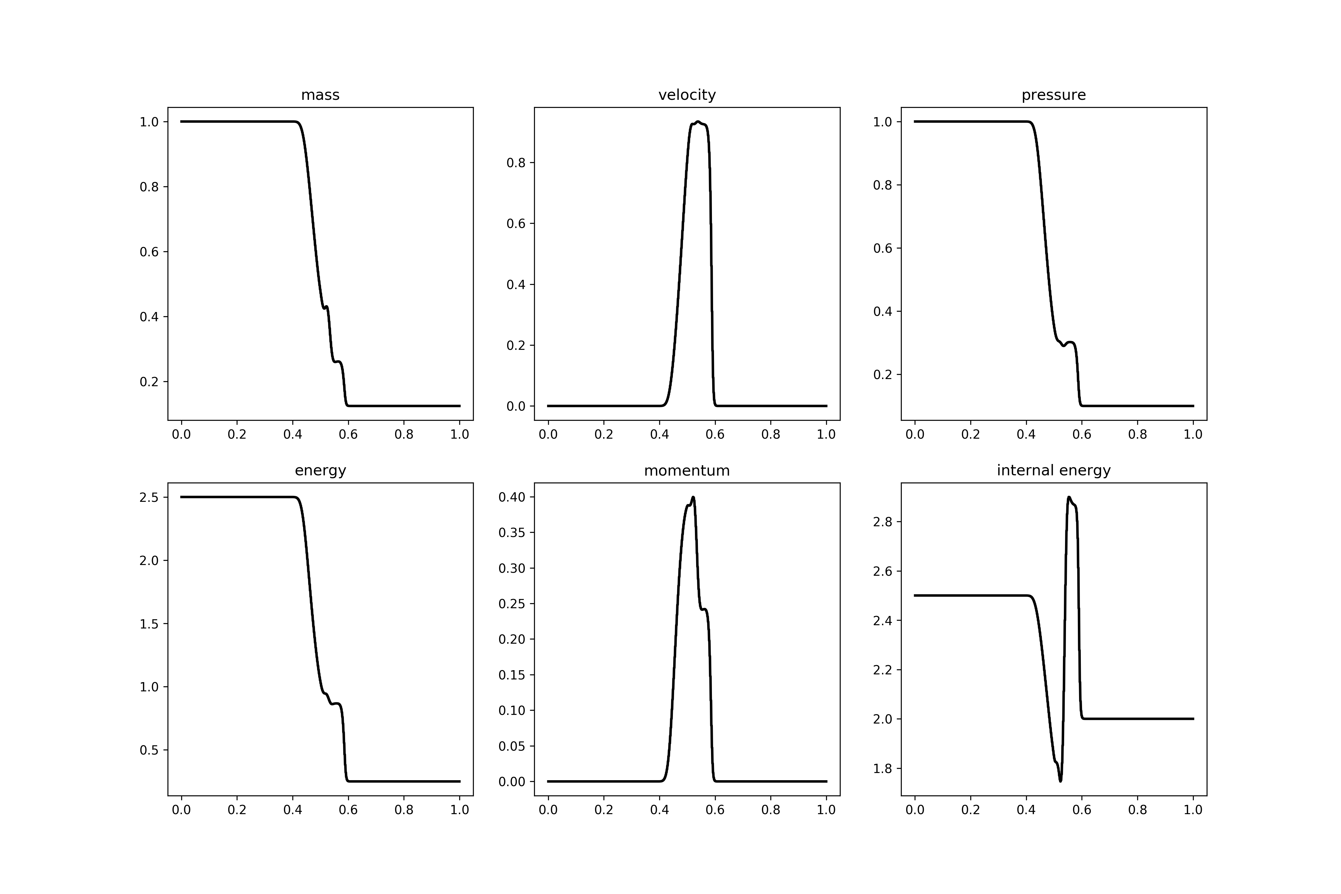
The most important classes
|
Create a geometry that defines the fluid part and the solid part. |
|
Create a domain that defines the fluid part and the solid part and computes the distances between these two states. |
|
Create the class with all the needed informations for each elementary scheme. |
|
create a class simulation |
The modules
|
Create the stencil of velocities used by the scheme(s). |
|
Create a stencil of a LBM scheme. |
|
Create a velocity. |
New in version 0.2: the geometrical elements are yet implemented in 3D.
The module elements contains all the geometrical shapes that can be used to build the geometry.
The 2D elements are:
|
Class Circle |
|
Class Ellipse |
|
Class Parallelogram |
|
Class Triangle |
The 3D elements are:
|
Class Sphere |
|
Class Ellipsoid |
|
Class Parallelepiped |
|
Class Cylinder_Circle |
|
Class Cylinder_Ellipse |
|
Class Cylinder_Triangle |
|
Create a geometry that defines the fluid part and the solid part. |
|
Create a domain that defines the fluid part and the solid part and computes the distances between these two states. |
|
This class defines the storage of the moments and distribution functions in pylbm. |
|
This class defines a structure of arrays to store the unknowns of the lattice Boltzmann schemes. |
|
This class defines an array of structures to store the unknowns of the lattice Boltzmann schemes. |
The module bounds contains the classes needed to treat the boundary conditions with the LBM formalism
The classes are
|
Construct the boundary problem by defining the list of indices on the border and the methods used on each label. |
|
Set boundary method. |
|
Boundary condition of type bounce-back |
|
Boundary condition of type anti bounce-back |
|
Boundary condition of type Neumann |
D. D’HUMIERES, Generalized Lattice-Boltzmann Equations, Rarefied Gas Dynamics: Theory and Simulations, 159, pp. 450-458, AIAA Progress in astronomics and aeronautics (1992).
F. DUBOIS, Equivalent partial differential equations of a lattice Boltzmann scheme, Computers and Mathematics with Applications, 55, pp. 1441-1449 (2008).
B. GRAILLE, Approximation of mono-dimensional hyperbolic systems: a lattice Boltzmann scheme as a relaxation method, Journal of Comutational Physics, 266 (3179757), pp. 74-88 (2014).
Y.H. QIAN, D. D’HUMIERES, and P. LALLEMAND, Lattice BGK Models for Navier-Stokes Equation, Europhys. Lett., 17 (6), pp. 479-484 (1992).


