In this tutorial, we consider the classical \(\DdQq{2}{9}\) to simulate a Poiseuille flow modeling by the Navier-Stokes equations.
[1]:
from __future__ import print_function, division
from six.moves import range
%matplotlib inline
In the following, we build the dictionary of the simulation step by step.
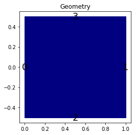
The simulation is done on a rectangle of length \(L\) and width \(W\). We can use \(L=W=1\).
We propose a dictionary that build the geometry of the domain. The labels of the bounds can be specified to different values for the moment.
[2]:
import numpy as np
import matplotlib.pyplot as plt

import pylbm

L, W = 1., 1.
dico_geom = {'box':{'x':[0,L], 'y':[-.5*W,.5*W], 'label':list(range(4))}}
geom = pylbm.Geometry(dico_geom)
print(geom)
geom.visualize(viewlabel=True)
/home/loic/miniconda3/envs/pylbm/lib/python3.6/site-packages/h5py/__init__.py:36: FutureWarning: Conversion of the second argument of issubdtype from `float` to `np.floating` is deprecated. In future, it will be treated as `np.float64 == np.dtype(float).type`.
  from ._conv import register_converters as _register_converters
Geometry informations
         spatial dimension: 2
         bounds of the box:
[[ 0.   1. ]
 [-0.5  0.5]]
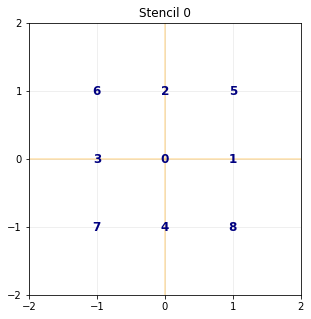
The stencil of the \(\DdQq{2}{9}\) is composed by the nine following velocities in 2D:
[3]:
dico_sten = {
    'dim':2,
    'schemes':[{'velocities':list(range(9))}],
}
sten = pylbm.Stencil(dico_sten)
print(sten)
sten.visualize()
Stencil informations
         * spatial dimension: 2
         * maximal velocity in each direction: [1 1]
         * minimal velocity in each direction: [-1 -1]
         * Informations for each elementary stencil:
                stencil 0
                 - number of velocities:  9
                 - velocities: (0: 0, 0), (1: 1, 0), (2: 0, 1), (3: -1, 0), (4: 0, -1), (5: 1, 1), (6: -1, 1), (7: -1, -1), (8: 1, -1),
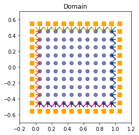
In order to build the domain of the simulation, the dictionary should contain the space step \(\dx\) and the stencils of the velocities (one for each scheme).
[4]:
dico_dom = {
    'space_step':.1,
    'box':{'x':[0,L], 'y':[-.5*W,.5*W], 'label':list(range(4))},
    'schemes':[{'velocities':list(range(9))}],
}
dom = pylbm.Domain(dico_dom)
print(dom)
dom.visualize(view_distance=True)
Domain informations
         spatial dimension: 2
         space step: dx= 1.000e-01
In pylbm, a simulation can be performed by using several coupled schemes. In this example, a single scheme is used and defined through a list of one single dictionary. This dictionary should contain:
‘velocities’: a list of the velocities
‘conserved_moments’: a list of the conserved moments as sympy variables
‘polynomials’: a list of the polynomials that define the moments
‘equilibrium’: a list of the equilibrium value of all the moments
‘relaxation_parameters’: a list of the relaxation parameters (\(0\) for the conserved moments)
‘init’: a dictionary to initialize the conserved moments
(see the documentation for more details)
In order to fix the bulk (\(\mu\)) and the shear (\(\eta\)) viscosities, we impose
The scheme velocity could be taken to \(1\) and the inital value of \(\rho\) to \(\rho_0=1\), \(q_x\) and \(q_y\) to \(0\).
In order to accelerate the simulation, we can use another generator. The default generator is Numpy (pure python). We can use for instance Cython that generates a more efficient code. This generator can be activated by using ‘generator’: pylbm.generator.CythonGenerator in the dictionary.
[5]:
import sympy as sp
X, Y, rho, qx, qy, LA = sp.symbols('X, Y, rho, qx, qy, LA')

# parameters
dx = 1./128  # spatial step
la = 1.      # velocity of the scheme
L = 1        # length of the domain
W = 1        # width of the domain
rhoo = 1.    # mean value of the density
mu   = 1.e-3 # shear viscosity
eta = 1.e-1 # bulk viscosity
# initialization
xmin, xmax, ymin, ymax = 0.0, L, -0.5*W, 0.5*W
dummy = 3.0/(la*rhoo*dx)
s_mu = 1.0/(0.5+mu*dummy)
s_eta = 1.0/(0.5+eta*dummy)
s_q = s_eta
s_es = s_mu
s  = [0.,0.,0.,s_mu,s_es,s_q,s_q,s_eta,s_eta]
dummy = 1./(LA**2*rhoo)
qx2 = dummy*qx**2
qy2 = dummy*qy**2
q2  = qx2+qy2
qxy = dummy*qx*qy

dico_sch = {
    'box':{'x':[xmin, xmax], 'y':[ymin, ymax], 'label':0},
    'space_step':dx,
    'scheme_velocity':la,
    'parameters':{LA:la},
    'schemes':[
        {
            'velocities':list(range(9)),
            'conserved_moments':[rho, qx, qy],
            'polynomials':[
                1, LA*X, LA*Y,
                3*(X**2+Y**2)-4,
                (9*(X**2+Y**2)**2-21*(X**2+Y**2)+8)/2,
                3*X*(X**2+Y**2)-5*X, 3*Y*(X**2+Y**2)-5*Y,
                X**2-Y**2, X*Y
            ],
            'relaxation_parameters':s,
            'equilibrium':[
                rho, qx, qy,
                -2*rho + 3*q2,
                rho-3*q2,
                -qx/LA, -qy/LA,
                qx2-qy2, qxy
            ],
            'init':{rho:rhoo, qx:0., qy:0.},
        },
    ],
    'generator': 'cython',
}
sch = pylbm.Scheme(dico_sch)
print(sch)
Scheme informations
         spatial dimension: dim=2
         number of schemes: nscheme=1
         number of velocities:
    Stencil.nv[0]=9
         velocities value:
    v[0] = (0: 0, 0), (1: 1, 0), (2: 0, 1), (3: -1, 0), (4: 0, -1), (5: 1, 1), (6: -1, 1), (7: -1, -1), (8: 1, -1),
         polynomials:
    P[0] = 1, LA*X, LA*Y, 3*X**2 + 3*Y**2 - 4, -21*X**2/2 - 21*Y**2/2 + 9*(X**2 + Y**2)**2/2 + 4, 3*X*(X**2 + Y**2) - 5*X, 3*Y*(X**2 + Y**2) - 5*Y, X**2 - Y**2, X*Y,
         equilibria:
    EQ[0] = rho, qx, qy, -2*rho + 3.0*qx**2/LA**2 + 3.0*qy**2/LA**2, rho - 3.0*qx**2/LA**2 - 3.0*qy**2/LA**2, -qx/LA, -qy/LA, 1.0*qx**2/LA**2 - 1.0*qy**2/LA**2, 1.0*qx*qy/LA**2,
         relaxation parameters:
    s[0] = 0.0, 0.0, 0.0, 1.13122171945701, 1.13122171945701, 0.0257069408740360, 0.0257069408740360, 0.0257069408740360, 0.0257069408740360,
         moments matrices
M      = Matrix([[1, 1, 1, 1, 1, 1, 1, 1, 1], [0, 1.0*LA, 0, -1.0*LA, 0, 1.0*LA, -1.0*LA, -1.0*LA, 1.0*LA], [0, 0, 1.0*LA, 0, -1.0*LA, 1.0*LA, 1.0*LA, -1.0*LA, -1.0*LA], [-4, -1.00000000000000, -1.00000000000000, -1.00000000000000, -1.00000000000000, 2.00000000000000, 2.00000000000000, 2.00000000000000, 2.00000000000000], [4, -2.00000000000000, -2.00000000000000, -2.00000000000000, -2.00000000000000, 1.00000000000000, 1.00000000000000, 1.00000000000000, 1.00000000000000], [0, -2.00000000000000, 0, 2.00000000000000, 0, 1.00000000000000, -1.00000000000000, -1.00000000000000, 1.00000000000000], [0, 0, -2.00000000000000, 0, 2.00000000000000, 1.00000000000000, 1.00000000000000, -1.00000000000000, -1.00000000000000], [0, 1.00000000000000, -1.00000000000000, 1.00000000000000, -1.00000000000000, 0, 0, 0, 0], [0, 0, 0, 0, 0, 1.00000000000000, -1.00000000000000, 1.00000000000000, -1.00000000000000]])
M^(-1) = Matrix([[0.111111111111111, 0, 0, -0.111111111111111, 0.111111111111111, 0, 0, 0, 0], [0.111111111111111, 0.166666666666667/LA, 0, -0.0277777777777778, -0.0555555555555556, -0.166666666666667, 0, 0.250000000000000, 0], [0.111111111111111, 0, 0.166666666666667/LA, -0.0277777777777778, -0.0555555555555556, 0, -0.166666666666667, -0.250000000000000, 0], [0.111111111111111, -0.166666666666667/LA, 0, -0.0277777777777778, -0.0555555555555556, 0.166666666666667, 0, 0.250000000000000, 0], [0.111111111111111, 0, -0.166666666666667/LA, -0.0277777777777778, -0.0555555555555556, 0, 0.166666666666667, -0.250000000000000, 0], [0.111111111111111, 0.166666666666667/LA, 0.166666666666667/LA, 0.0555555555555556, 0.0277777777777778, 0.0833333333333333, 0.0833333333333333, 0, 0.250000000000000], [0.111111111111111, -0.166666666666667/LA, 0.166666666666667/LA, 0.0555555555555556, 0.0277777777777778, -0.0833333333333333, 0.0833333333333333, 0, -0.250000000000000], [0.111111111111111, -0.166666666666667/LA, -0.166666666666667/LA, 0.0555555555555556, 0.0277777777777778, -0.0833333333333333, -0.0833333333333333, 0, 0.250000000000000], [0.111111111111111, 0.166666666666667/LA, -0.166666666666667/LA, 0.0555555555555556, 0.0277777777777778, 0.0833333333333333, -0.0833333333333333, 0, -0.250000000000000]])
For the simulation, we take
The domain \(x\in(0, L)\) and \(y\in(-W/2,W/2)\), \(L=2\), \(W=1\),
the viscosities \(\mu=10^{-2}=\eta=10^{-2}\),
the space step \(\dx=1/128\), the scheme velocity \(\lambda=1\),
the mean density \(\rho_0=1\).
Concerning the boundary conditions, we impose the velocity on all the edges by a bounce-back condition with a source term that reads
with \(v_{\text{max}}=0.1\).
We compute the solution for \(t\in(0,50)\) and we plot several slices of the solution during the simulation.
This problem has an exact solution given by
where the pressure gradient \(K\) reads
We compute the exact and the numerical gradients of the pressure.
[6]:
X, Y, LA = sp.symbols('X, Y, LA')
rho, qx, qy = sp.symbols('rho, qx, qy')

def bc(f, m, x, y):
    m[qx] = rhoo * vmax * (1.-4.*y**2/W**2)
    m[qy] = 0.

def plot_coupe(sol):
    fig, ax1 = plt.subplots()
    ax2 = ax1.twinx()
    ax1.cla()
    ax2.cla()
    mx = int(sol.domain.shape_in[0]/2)
    my = int(sol.domain.shape_in[1]/2)
    x = sol.domain.x
    y = sol.domain.y
    u = sol.m[qx] / rhoo
    for i in [0,mx,-1]:
        ax1.plot(y+x[i], u[i, :], 'b')
    for j in [0,my,-1]:
        ax1.plot(x+y[j], u[:,j], 'b')
    ax1.set_ylabel('velocity', color='b')
    for tl in ax1.get_yticklabels():
        tl.set_color('b')
    ax1.set_ylim(-.5*rhoo*vmax, 1.5*rhoo*vmax)
    p = sol.m[rho][:,my] * la**2 / 3.0
    p -= np.average(p)
    ax2.plot(x, p, 'r')
    ax2.set_ylabel('pressure', color='r')
    for tl in ax2.get_yticklabels():
        tl.set_color('r')
    ax2.set_ylim(pressure_gradient*L, -pressure_gradient*L)
    plt.title('Poiseuille flow at t = {0:f}'.format(sol.t))
    plt.draw()
    plt.pause(1.e-3)

# parameters
dx = 1./16  # spatial step
la = 1.      # velocity of the scheme
Tf = 50      # final time of the simulation
L = 2        # length of the domain
W = 1        # width of the domain
vmax = 0.1   # maximal velocity obtained in the middle of the channel
rhoo = 1.    # mean value of the density
mu = 1.e-2   # bulk viscosity
eta = 1.e-2  # shear viscosity
pressure_gradient = - vmax * 8.0 / W**2 * eta
# initialization
xmin, xmax, ymin, ymax = 0.0, L, -0.5*W, 0.5*W
dummy = 3.0/(la*rhoo*dx)
s_mu = 1.0/(0.5+mu*dummy)
s_eta = 1.0/(0.5+eta*dummy)
s_q = s_eta
s_es = s_mu
s  = [0.,0.,0.,s_mu,s_es,s_q,s_q,s_eta,s_eta]
dummy = 1./(LA**2*rhoo)
qx2 = dummy*qx**2
qy2 = dummy*qy**2
q2  = qx2+qy2
qxy = dummy*qx*qy

dico = {
    'box':{'x':[xmin, xmax], 'y':[ymin, ymax], 'label':0},
    'space_step':dx,
    'scheme_velocity':la,
    'parameters':{LA:la},
    'schemes':[
        {
            'velocities':list(range(9)),
            'conserved_moments':[rho, qx, qy],
            'polynomials':[
                1, LA*X, LA*Y,
                3*(X**2+Y**2)-4,
                (9*(X**2+Y**2)**2-21*(X**2+Y**2)+8)/2,
                3*X*(X**2+Y**2)-5*X, 3*Y*(X**2+Y**2)-5*Y,
                X**2-Y**2, X*Y
            ],
            'relaxation_parameters':s,
            'equilibrium':[
                rho, qx, qy,
                -2*rho + 3*q2,
                rho-3*q2,
                -qx/LA, -qy/LA,
                qx2-qy2, qxy
            ],
            'init':{rho:rhoo, qx:0., qy:0.},
        },
    ],
    'boundary_conditions':{
        0:{'method':{0: pylbm.bc.Bouzidi_bounce_back}, 'value':bc}
    },
    'generator': 'cython',
}

sol = pylbm.Simulation(dico)
while (sol.t<Tf):
    sol.one_time_step()
plot_coupe(sol)
ny = int(sol.domain.shape_in[1]/2)
num_pressure_gradient = (sol.m[rho][-2,ny] - sol.m[rho][1,ny]) / (xmax-xmin) * la**2/ 3.0
print("Exact pressure gradient    : {0:10.3e}".format(pressure_gradient))
print("Numerical pressure gradient: {0:10.3e}".format(num_pressure_gradient))
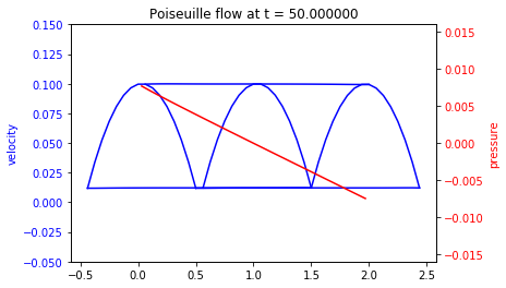
Exact pressure gradient    : -8.000e-03
Numerical pressure gradient: -7.074e-03
[ ]: