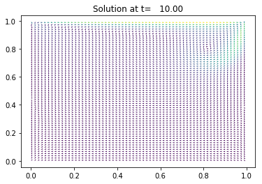
In this tutorial, we consider the classical \(\DdQq{2}{9}\) and \(\DdQq{3}{15}\) to simulate a lid driven acvity modeling by the Navier-Stokes equations. The \(\DdQq{2}{9}\) is used in dimension \(2\) and the \(\DdQq{3}{15}\) in dimension \(3\).
[1]:
from __future__ import print_function, division
from six.moves import range
%matplotlib inline
The \(\DdQq{2}{9}\) is defined by:
a space step \(\dx\) and a time step \(\dt\) related to the scheme velocity \(\lambda\) by the relation \(\lambda=\dx/\dt\),
nine velocities \(\{(0,0), (\pm1,0), (0,\pm1), (\pm1, \pm1)\}\), identified in pylbm by the numbers \(0\) to \(8\),
nine polynomials used to build the moments
where \(E = X^2+Y^2\).
three conserved moments \(\rho\), \(q_x\), and \(q_y\),
nine relaxation parameters (three are \(0\) corresponding to conserved moments): \(\{0,0,0,s_\mu,s_\mu,s_\eta,s_\eta,s_\eta,s_\eta\}\), where \(s_\mu\) and \(s_\eta\) are in \((0,2)\),
equilibrium value of the non conserved moments
where \(\rho_0\) is a given scalar.
This scheme is consistant at second order with the following equations (taken \(\rho_0=1\))
with \(p=\rho\lambda^2/3\).
We write the dictionary for a simulation of the Navier-Stokes equations on \((0,1)^2\).
In order to impose the boundary conditions, we use the bounce-back conditions to fix \(q_x=q_y=0\) at south, east, and west and \(q_x=\rho u\), \(q_y=0\) at north. The driven velocity \(u\) could be \(u=\lambda/10\).
The solution is governed by the Reynolds number \(Re = \rho_0u / \eta\). We fix the relaxation parameters to have \(Re=1000\). The relaxation parameters related to the bulk viscosity \(\mu\) should be large enough to ensure the stability (for instance \(\mu=10^{-3}\)).
We compute the stationary solution of the problem obtained for large enough final time. We plot the solution with the function quiver of matplotlib.
[2]:
import numpy as np
import sympy as sp
import matplotlib.pyplot as plt
import pylbm

X, Y, LA = sp.symbols('X, Y, LA')
rho, qx, qy = sp.symbols('rho, qx, qy')

def bc(f, m, x, y):
    m[qx] = rhoo * vup

def plot(sol):
    pas = 2
    y, x = np.meshgrid(sol.domain.y[::pas], sol.domain.x[::pas])
    u = sol.m[qx][::pas,::pas] / sol.m[rho][::pas,::pas]
    v = sol.m[qy][::pas,::pas] / sol.m[rho][::pas,::pas]
    nv = np.sqrt(u**2+v**2)
    normu = nv.max()
    u = u / (nv+1e-5)
    v = v / (nv+1e-5)
    plt.quiver(x, y, u, v, nv, pivot='mid')
    plt.title('Solution at t={0:8.2f}'.format(sol.t))
    plt.show()

# parameters
Re = 1000
dx = 1./128  # spatial step
la = 1.      # velocity of the scheme
Tf = 10      # final time of the simulation
vup = la/5   # maximal velocity obtained in the middle of the channel
rhoo = 1.    # mean value of the density
mu = 1.e-4   # bulk viscosity
eta = rhoo*vup/Re  # shear viscosity
# initialization
xmin, xmax, ymin, ymax = 0., 1., 0., 1.
dummy = 3.0/(la*rhoo*dx)
s_mu = 1.0/(0.5+mu*dummy)
s_eta = 1.0/(0.5+eta*dummy)
s_q = s_eta
s_es = s_mu
s  = [0.,0.,0.,s_mu,s_es,s_q,s_q,s_eta,s_eta]
dummy = 1./(LA**2*rhoo)
qx2 = dummy*qx**2
qy2 = dummy*qy**2
q2  = qx2+qy2
qxy = dummy*qx*qy

print("Reynolds number: {0:10.3e}".format(Re))
print("Bulk viscosity : {0:10.3e}".format(mu))
print("Shear viscosity: {0:10.3e}".format(eta))
print("relaxation parameters: {0}".format(s))

dico = {
    'box':{'x':[xmin, xmax], 'y':[ymin, ymax], 'label':[0,0,0,1]},
    'space_step':dx,
    'scheme_velocity':la,
    'parameters':{LA:la},
    'schemes':[
        {
            'velocities':list(range(9)),
            'conserved_moments':[rho, qx, qy],
            'polynomials':[
                1, LA*X, LA*Y,
                3*(X**2+Y**2)-4,
                0.5*(9*(X**2+Y**2)**2-21*(X**2+Y**2)+8),
                3*X*(X**2+Y**2)-5*X, 3*Y*(X**2+Y**2)-5*Y,
                X**2-Y**2, X*Y
            ],
            'relaxation_parameters':s,
            'equilibrium':[
                rho, qx, qy,
                -2*rho + 3*q2,
                rho-3*q2,
                -qx/LA, -qy/LA,
                qx2-qy2, qxy
            ],
            'init':{rho:rhoo, qx:0., qy:0.},
        },
    ],
    'boundary_conditions':{
        0:{'method':{0: pylbm.bc.Bouzidi_bounce_back}, 'value':None},
        1:{'method':{0: pylbm.bc.Bouzidi_bounce_back}, 'value':bc}
    },
    'generator': 'cython',
}

sol = pylbm.Simulation(dico)
while (sol.t<Tf):
    sol.one_time_step()
plot(sol)
/home/loic/miniconda3/envs/pylbm/lib/python3.6/site-packages/h5py/__init__.py:36: FutureWarning: Conversion of the second argument of issubdtype from `float` to `np.floating` is deprecated. In future, it will be treated as `np.float64 == np.dtype(float).type`.
  from ._conv import register_converters as _register_converters
Reynolds number:  1.000e+03
Bulk viscosity :  1.000e-04
Shear viscosity:  2.000e-04
relaxation parameters: [0.0, 0.0, 0.0, 1.8573551263001487, 1.8573551263001487, 1.7337031900138697, 1.7337031900138697, 1.7337031900138697, 1.7337031900138697]
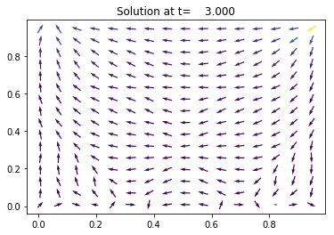
The \(\DdQq{3}{15}\) is defined by:
a space step \(\dx\) and a time step \(\dt\) related to the scheme velocity \(\lambda\) by the relation \(\lambda=\dx/\dt\),
fifteen velocities \(\{(0,0,0), (\pm1,0,0), (0,\pm1,0), (0,0,\pm1), (\pm1, \pm1,\pm1)\}\), identified in pylbm by the numbers \(\{0,\ldots,6,19,\ldots,26\}\),
fifteen polynomials used to build the moments
where \(E = X^2+Y^2+Z^2\).
four conserved moments \(\rho\), \(q_x\), \(q_y\), and \(q_z\),
fifteen relaxation parameters (four are \(0\) corresponding to conserved moments): \(\{0, s_1, s_2, 0, s_4, 0, s_4, 0, s_4, s_9, s_9, s_{11}, s_{11}, s_{11}, s_{14}\}\),
equilibrium value of the non conserved moments
This scheme is consistant at second order with the Navier-Stokes equations with the shear viscosity \(\eta\) and the relaxation parameter \(s_9\) linked by the relation
We write a dictionary for a simulation of the Navier-Stokes equations on \((0,1)^3\).
In order to impose the boundary conditions, we use the bounce-back conditions to fix \(q_x=q_y=q_z=0\) at south, north, east, west, and bottom and \(q_x=\rho u\), \(q_y=q_z=0\) at top. The driven velocity \(u\) could be \(u=\lambda/10\).
We compute the stationary solution of the problem obtained for large enough final time. We plot the solution with the function quiver of matplotlib.
[3]:
X, Y, Z, LA = sp.symbols('X, Y, Z, LA')
rho, qx, qy, qz = sp.symbols('rho, qx, qy, qz')

def bc(f, m, x, y, z):
    m[qx] = rhoo * vup

def plot(sol):
    plt.clf()
    pas = 4
    nz = int(sol.domain.shape_in[1] / 2) + 1
    y, x = np.meshgrid(sol.domain.y[::pas], sol.domain.x[::pas])
    u = sol.m[qx][::pas,nz,::pas] / sol.m[rho][::pas,nz,::pas]
    v = sol.m[qz][::pas,nz,::pas] / sol.m[rho][::pas,nz,::pas]
    nv = np.sqrt(u**2+v**2)
    normu = nv.max()
    u = u / (nv+1e-5)
    v = v / (nv+1e-5)
    plt.quiver(x, y, u, v, nv, pivot='mid')
    plt.title('Solution at t={0:9.3f}'.format(sol.t))
    plt.show()

# parameters
Re = 2000
dx = 1./64   # spatial step
la = 1.      # velocity of the scheme
Tf = 3       # final time of the simulation
vup = la/10  # maximal velocity obtained in the middle of the channel
rhoo = 1.    # mean value of the density
eta = rhoo*vup/Re  # shear viscosity
# initialization
xmin, xmax, ymin, ymax, zmin, zmax = 0., 1., 0., 1., 0., 1.
dummy = 3.0/(la*rhoo*dx)

s1 = 1.6
s2 = 1.2
s4 = 1.6
s9 = 1./(.5+dummy*eta)
s11 = s9
s14 = 1.2
s  = [0, s1, s2, 0, s4, 0, s4, 0, s4, s9, s9, s11, s11, s11, s14]

r = X**2+Y**2+Z**2

print("Reynolds number: {0:10.3e}".format(Re))
print("Shear viscosity: {0:10.3e}".format(eta))

dico = {
    'box':{
        'x':[xmin, xmax],
        'y':[ymin, ymax],
        'z':[zmin, zmax],
        'label':[0,0,0,0,0,1]
    },
    'space_step':dx,
    'scheme_velocity':la,
    'parameters':{LA:la},
    'schemes':[
        {
            'velocities':list(range(7)) + list(range(19,27)),
            'conserved_moments':[rho, qx, qy, qz],
            'polynomials':[
                1,
                r - 2, .5*(15*r**2-55*r+32),
                X, .5*(5*r-13)*X,
                Y, .5*(5*r-13)*Y,
                Z, .5*(5*r-13)*Z,
                3*X**2-r, Y**2-Z**2,
                X*Y, Y*Z, Z*X,
                X*Y*Z
            ],
            'relaxation_parameters':s,
            'equilibrium':[
                rho,
                -rho + qx**2 + qy**2 + qz**2,
                -rho,
                qx,
                -7./3*qx,
                qy,
                -7./3*qy,
                qz,
                -7./3*qz,
                1./3*(2*qx**2-(qy**2+qz**2)),
                qy**2-qz**2,
                qx*qy,
                qy*qz,
                qz*qx,
                0
            ],
            'init':{rho:rhoo, qx:0., qy:0., qz:0.},
        },
    ],
    'boundary_conditions':{
        0:{'method':{0: pylbm.bc.Bouzidi_bounce_back}, 'value':None},
        1:{'method':{0: pylbm.bc.Bouzidi_bounce_back}, 'value':bc}
    },
    'generator': 'cython',
}

sol = pylbm.Simulation(dico)
while (sol.t<Tf):
    sol.one_time_step()
plot(sol)
Reynolds number:  2.000e+03
Shear viscosity:  5.000e-05
[ ]: