Transport equation with source term¶

\[\renewcommand{\DdQq}[2]{{\mathrm D}_{#1}{\mathrm Q}_{#2}} \renewcommand{\drondt}{\partial_t} \renewcommand{\drondx}{\partial_x} \renewcommand{\dx}{\Delta x} \renewcommand{\dt}{\Delta t} \renewcommand{\grandO}{{\mathcal O}} \renewcommand{\density}[2]{\,f_{#1}^{#2}} \renewcommand{\fk}[1]{\density{#1}{\vphantom{\star}}} \renewcommand{\fks}[1]{\density{#1}{\star}} \renewcommand{\moment}[2]{\,m_{#1}^{#2}} \renewcommand{\mk}[1]{\moment{#1}{\vphantom{\star}}} \renewcommand{\mke}[1]{\moment{#1}{e}} \renewcommand{\mks}[1]{\moment{#1}{\star}}\]

In this tutorial, we propose to add a source term in the advection equation. The problem reads

\[\drondt u + c \drondx u = S(t, x, u), \quad t>0, , \quad x\in(0, 1),\]

where \(c\) is a constant scalar (typically \(c=1\)). Additional boundary and initial conditions will be given in the following. \(S\) is the source term that can depend on the time \(t\), the space \(x\) and the solution \(u\).

In order to simulate this problem, we use the \(\DdQq{1}{2}\) scheme and we add an additional key:value in the dictionary for the source term. We deal with two examples.

A friction term¶

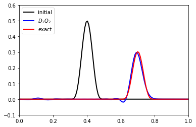
In this example, we takes \(S(t, x, u) = -\alpha u\) where \(\alpha\) is a positive constant. The dictionary of the simulation then reads:

[1]:

%matplotlib inline
import sympy as sp
import numpy as np
import pylbm

[2]:

C, ALPHA, X, u, LA = sp.symbols('C, ALPHA, X, u, LA')
c = 0.3
alpha = 0.5

def init(x):
    middle, width, height = 0.4, 0.1, 0.5
    return height/width**10 * (x%1-middle-width)**5 * \
                              (middle-x%1-width)**5 * (abs(x%1-middle)<=width)

def solution(t, x):
    return init(x - c*t)*np.exp(-alpha*t)

dico = {
    'box': {'x': [0., 1.], 'label': -1},
    'space_step': 1./128,
    'scheme_velocity': LA,
    'schemes': [
        {
            'velocities': [1,2],
            'conserved_moments': u,
            'polynomials': [1, LA*X],
            'relaxation_parameters': [0., 2.],
            'equilibrium': [u, C*u],
            'source_terms': {u: -ALPHA*u},
        },
    ],
    'init': {u: init},
    'parameters': {
        LA: 1.,
        C: c,
        ALPHA: alpha
    },
    'generator': 'numpy',
}

sol = pylbm.Simulation(dico) # build the simulation
viewer = pylbm.viewer.matplotlib_viewer
fig = viewer.Fig()
ax = fig[0]
ax.axis(0., 1., -.1, .6)
x = sol.domain.x
ax.plot(x, sol.m[u], width=2, color='k', label='initial')
while sol.t < 1:
    sol.one_time_step()
ax.plot(x, sol.m[u], width=2, color='b', label=r'$D_1Q_2$')
ax.plot(x, solution(sol.t, x), width=2, color='r', label='exact')
ax.legend()

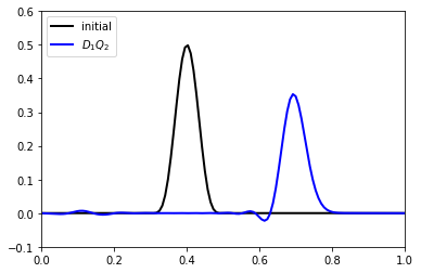
../_images/notebooks_08_advection_reaction_3_0.png

A source term depending on time and space¶

If the source term \(S\) depends explicitely on the time or on the space, we have to specify the corresponding variables in the dictionary through the key parameters. The time variable is prescribed by the key ‘time’. Moreover, sympy functions can be used to define the source term like in the following example. This example is just for testing the feature… no physical meaning in mind !

[3]:

t, C, X, u, LA = sp.symbols('t, C, X, u, LA')
c = 0.3

def init(x):
    middle, width, height = 0.4, 0.1, 0.5
    return height/width**10 * (x%1-middle-width)**5 * \
                              (middle-x%1-width)**5 * (abs(x%1-middle)<=width)

dico = {
    'box': {'x': [0., 1.], 'label': -1},
    'space_step': 1./128,
    'scheme_velocity': LA,
    'schemes': [
        {
            'velocities': [1, 2],
            'conserved_moments': u,
            'polynomials': [1, LA*X],
            'relaxation_parameters': [0., 2.],
            'equilibrium': [u, C*u],
            'source_terms': {u: -sp.Abs(X-t)**2*u},
        },
    ],
    'init': {u: init},
    'generator': 'cython',
    'parameters': {LA: 1., C: c},
}

sol = pylbm.Simulation(dico) # build the simulation
viewer = pylbm.viewer.matplotlib_viewer
fig = viewer.Fig()
ax = fig[0]
ax.axis(0., 1., -.1, .6)
x = sol.domain.x
ax.plot(x, sol.m[u], width=2, color='k', label='initial')
while sol.t < 1:
    sol.one_time_step()
ax.plot(x, sol.m[u], width=2, color='b', label=r'$D_1Q_2$')
ax.legend()

../_images/notebooks_08_advection_reaction_5_0.png