The Domain of the simulation¶

With pylbm, the numerical simulations can be performed in a domain with a complex geometry. The creation of the geometry from a dictionary is explained here. All the informations needed to build the domain are defined through a dictionary and put in a object of the class Domain.

The domain is built from three types of informations:

a geometry (class Geometry),
a stencil (class Stencil),
a space step (a float for the grid step of the simulation).

The domain is a uniform cartesian discretization of the geometry with a grid step \(dx\). The whole box is discretized even if some elements are added to reduce the domain of the computation. The stencil is necessary in order to know the maximal velocity in each direction so that the corresponding number of phantom cells are added at the borders of the domain (for the treatment of the boundary conditions). The user can get the coordinates of the points in the domain by the fields x, y, and z. By convention, if the spatial dimension is one, y=z=None; and if it is two, z=None.

Several examples of domains can be found in demo/examples/domain/

Examples in 1D¶

script

The segment \([0, 1]\) with a \(D_1Q_3\)¶

dico = {
    'box':{'x': [0, 1], 'label':0},
    'space_step':0.1,
    'schemes':[{'velocities':list(range(3))}],
}
dom = pylbm.Domain(dico)
dom.visualize()

(Source code, png, pdf)

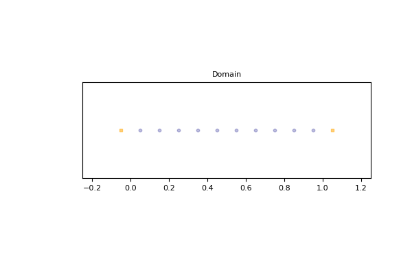
The segment \([0,1]\) is created by the dictionary with the key box. The stencil is composed by the velocity \(v_0=0\), \(v_1=1\), and \(v_2=-1\). One phantom cell is then added at the left and at the right of the domain. The space step \(dx\) is taken to \(0.1\) to allow the visualization. The result is then visualized with the distance of the boundary points by using the method visualize.

script

The segment \([0, 1]\) with a \(D_1Q_5\)¶

dico = {
    'box':{'x': [0, 1], 'label':0},
    'space_step':0.1,
    'schemes':[{'velocities':list(range(5))}],
}
dom = pylbm.Domain(dico)
dom.visualize()

(Source code, png, pdf)

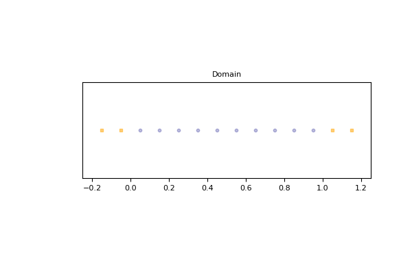
The segment \([0,1]\) is created by the dictionary with the key box. The stencil is composed by the velocity \(v_0=0\), \(v_1=1\), \(v_2=-1\), \(v_3=2\), \(v_4=-2\). Two phantom cells are then added at the left and at the right of the domain. The space step \(dx\) is taken to \(0.1\) to allow the visualization. The result is then visualized with the distance of the boundary points by using the method visualize.

Examples in 2D¶

script

The square \([0,1]^2\) with a \(D_2Q_9\)¶

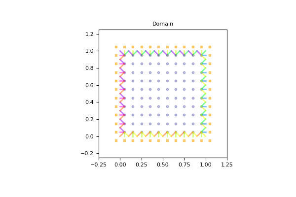
dico = {
    'box':{'x': [0, 1], 'y': [0, 1], 'label':0},
    'space_step':0.1,
    'schemes':[{'velocities':list(range(9))}],
}
dom = pylbm.Domain(dico)
dom.visualize()
dom.visualize(view_distance=True)

(Source code)

(png, pdf)¶

(png, pdf)¶

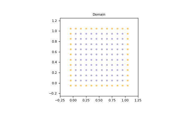
The square \([0,1]^2\) is created by the dictionary with the key box. The stencil is composed by the nine velocities

\begin{equation} \begin{gathered} v_0=(0,0),\\ v_1=(1,0), v_2=(0,1), v_3=(-1,0), v_4=(0,-1),\\ v_5=(1,1), v_6=(-1,1), v_7=(-1,-1), v_8=(1,-1). \end{gathered} \end{equation}

One phantom cell is then added all around the square. The space step \(dx\) is taken to \(0.1\) to allow the visualization. The result is then visualized by using the method visualize. This method can be used without parameter: the domain is visualize in white for the fluid part (where the computation is done) and in black for the solid part (the phantom cells or the obstacles). An optional parameter view_distance can be used to visualize more precisely the points (a black circle inside the domain and a square outside). Color lines are added to visualize the position of the border: for each point that can reach the border for a given velocity in one time step, the distance to the border is computed.

script 1

A square with a hole with a \(D_2Q_{13}\)¶

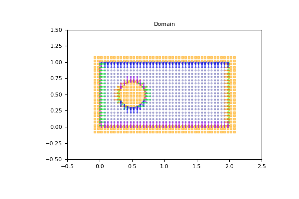
The unit square \([0,1]^2\) can be holed with a circle. In this example, a solid disc lies in the fluid domain defined by a circle with a center of (0.5, 0.5) and a radius of 0.125

dico = {
    'box':{'x': [0, 2], 'y': [0, 1], 'label':0},
    'elements':[pylbm.Circle((0.5,0.5), 0.2)],
    'space_step':0.05,
    'schemes':[{'velocities':list(range(13))}],
}
dom = pylbm.Domain(dico)
dom.visualize()
dom.visualize(view_distance=True)

(Source code)

(png, pdf)¶

(png, pdf)¶

script

A step with a \(D_2Q_9\)¶

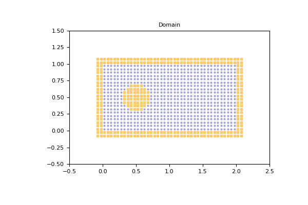
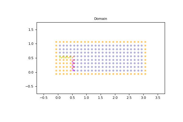
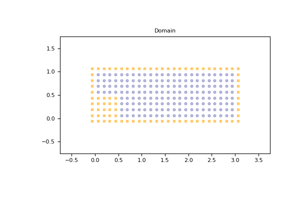
A step can be build by removing a rectangle in the left corner. For a \(D_2Q_9\), it gives the following domain.

dico = {
    'box':{'x': [0, 3], 'y': [0, 1], 'label':0},
    'elements':[pylbm.Parallelogram((0.,0.), (.5,0.), (0., .5), label=1)],
    'space_step':0.125,
    'schemes':[{'velocities':list(range(9))}],
}
dom = pylbm.Domain(dico)
dom.visualize()
dom.visualize(view_distance=True, label=1)

(Source code)

(png, pdf)¶

(png, pdf)¶

Note that the distance with the bound is visible only for the specified labels.

Examples in 3D¶

script

The cube \([0,1]^3\) with a \(D_3Q_{19}\)¶

dico = {
    'box':{'x': [0, 2], 'y': [0, 2], 'z':[0, 2], 'label':0},
    'space_step':.5,
    'schemes':[{'velocities':list(range(19))}]
}
dom = pylbm.Domain(dico)
dom.visualize()
dom.visualize(view_distance=True)

(Source code)

The cube \([0,1]^3\) is created by the dictionary with the key box and the first 19th velocities. The result is then visualized by using the method visualize.

The cube with a hole with a \(D_3Q_{19}\)¶

dico = {
    'box':{'x': [0, 2], 'y': [0, 2], 'z':[0, 2], 'label':0},
    'elements':[pylbm.Sphere((1,1,1), 0.5, label = 1)],
    'space_step':.5,
    'schemes':[{'velocities':list(range(19))}]
}
dom = pylbm.Domain(dico)
dom.visualize()
dom.visualize(view_distance=False, view_bound=True, label=1, view_in=False, view_out=False)

(Source code)