In this tutorial, we test a very classical lattice Boltzmann scheme \(\DdQq{1}{3}\) on the heat equation.
The problem reads
where \(\mu\) is a constant scalar.
[1]:
%matplotlib inline
The numerical simulation of this equation by a lattice Boltzmann scheme consists in the approximatation of the solution on discret points of \((0,1)\) at discret instants.
To simulate this system of equations, we use the \(\DdQq{1}{3}\) scheme given by
three velocities \(v_0=0\), \(v_1=1\), and \(v_2=-1\), with associated distribution functions \(\fk{0}\), \(\fk{1}\), and \(\fk{2}\),
a space step \(\dx\) and a time step \(\dt\), the ration \(\lambda=\dx/\dt\) is called the scheme velocity,
three moments
and their equilibrium values \(\mke{0}\), \(\mke{1}\), and \(\mke{2}\).
two relaxation parameters \(s_1\) and \(s_2\) lying in \([0,2]\).
In order to use the formalism of the package pylbm, we introduce the three polynomials that define the moments: \(P_0 = 1\), \(P_1=X\), and \(P_2=X^2/2\), such that
The transformation \((\fk{0}, \fk{1}, \fk{2})\mapsto(\mk{0},\mk{1}, \mk{2})\) is invertible if, and only if, the polynomials \((P_0,P_1,P_2)\) is a free set over the stencil of velocities.
The lattice Boltzmann method consists to compute the distribution functions \(\fk{0}\), \(\fk{1}\), and \(\fk{2}\) in each point of the lattice \(x\) and at each time \(t^n=n\dt\). A step of the scheme can be read as a splitting between the relaxation phase and the transport phase:
relaxation:
m2f:
transport:
f2m:
The moment of order \(0\), \(\mk{0}\), being conserved during the relaxation phase, a diffusive scaling \(\dt=\dx^2\), yields to the following equivalent equation
if \(\mke{1}=0\). In order to be consistent with the heat equation, the following choice is done:
pylbm uses Python dictionary to describe the simulation. In the following, we will build this dictionary step by step.
In pylbm, the geometry is defined by a box and a label for the boundaries.
[2]:
import pylbm
import numpy as np

xmin, xmax = 0., 1.
dico_geom = {
    'box': {'x': [xmin, xmax], 'label':0},
}
geom = pylbm.Geometry(dico_geom)
print(geom)
geom.visualize(viewlabel=True);
+----------------------+
| Geometry information |
+----------------------+
    - spatial dimension: 1
    - bounds of the box: [0. 1.]
    - labels: [0, 0]
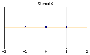
pylbm provides a class stencil that is used to define the discret velocities of the scheme. In this example, the stencil is composed by the velocities \(v_0=0\), \(v_1=1\) and \(v_2=-1\) numbered by \([0,1,2]\).
[3]:
dico_sten = {
    'dim': 1,
    'schemes':[{'velocities': list(range(3))}],
}
sten = pylbm.Stencil(dico_sten)
print(sten)
sten.visualize();
+---------------------+
| Stencil information |
+---------------------+
    - spatial dimension: 1
    - minimal velocity in each direction: [-1]
    - maximal velocity in each direction: [1]
    - information for each elementary stencil:
        stencil 0
            - number of velocities: 3
            - velocities
                (0: 0)
                (1: 1)
                (2: -1)
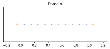
In order to build the domain of the simulation, the dictionary should contain the space step \(\dx\) and the stencils of the velocities (one for each scheme).
We construct a domain with \(N=10\) points in space.
[4]:
N = 10
dx = (xmax-xmin)/N
dico_dom = {
    'box': {'x': [xmin, xmax], 'label':0},
    'space_step': dx,
    'schemes': [
        {
            'velocities': list(range(3)),
        }
    ],
}
dom = pylbm.Domain(dico_dom)
print(dom)
dom.visualize();
+--------------------+
| Domain information |
+--------------------+
    - spatial dimension: 1
    - space step: 0.1
    - with halo:
        bounds of the box: [-0.05] x [1.05]
        number of points: [12]
    - without halo:
        bounds of the box: [0.05] x [0.95]
        number of points: [10]

    +----------------------+
    | Geometry information |
    +----------------------+
        - spatial dimension: 1
        - bounds of the box: [0. 1.]
        - labels: [0, 0]
In pylbm, a simulation can be performed by using several coupled schemes. In this example, a single scheme is used and defined through a list of one single dictionary. This dictionary should contain:
‘velocities’: a list of the velocities
‘conserved_moments’: a list of the conserved moments as sympy variables
‘polynomials’: a list of the polynomials that define the moments
‘equilibrium’: a list of the equilibrium value of all the moments
‘relaxation_parameters’: a list of the relaxation parameters (\(0\) for the conserved moments)
‘init’: a dictionary to initialize the conserved moments
(see the documentation for more details)
The scheme velocity could be taken to \(1/\dx\) and the inital value of \(u\) to
[5]:
import sympy as sp

def solution(x, t):
    return np.sin(np.pi*x)*np.exp(-np.pi**2*mu*t)

# parameters
mu = 1.
la = 1./dx
s1 = 2./(1+2*mu)
s2 = 1.
u, X = sp.symbols('u, X')

dico_sch = {
    'dim': 1,
    'scheme_velocity': la,
    'schemes':[
        {
            'velocities': list(range(3)),
            'conserved_moments': u,
            'polynomials': [1, X, X**2/2],
            'equilibrium': [u, 0., .5*u],
            'relaxation_parameters': [0., s1, s2],
        }
    ],
}

sch = pylbm.Scheme(dico_sch)
print(sch)
+--------------------+
| Scheme information |
+--------------------+
    - spatial dimension: 1
    - number of schemes: 1
    - number of velocities: 3
    - conserved moments: [u]

    +----------+
    | Scheme 0 |
    +----------+
        - velocities
            (0: 0)
            (1: 1)
            (2: -1)

        - polynomials

            ⎡1 ⎤
            ⎢  ⎥
            ⎢X ⎥
            ⎢  ⎥
            ⎢ 2⎥
            ⎢X ⎥
            ⎢──⎥
            ⎣2 ⎦

        - equilibria

            ⎡  u  ⎤
            ⎢     ⎥
            ⎢ 0.0 ⎥
            ⎢     ⎥
            ⎣0.5⋅u⎦

        - relaxation parameters

            ⎡       0.0       ⎤
            ⎢                 ⎥
            ⎢0.666666666666667⎥
            ⎢                 ⎥
            ⎣       1.0       ⎦

    - moments matrices

        ⎡1  1    1 ⎤
        ⎢          ⎥
        ⎢0  10  -10⎥
        ⎢          ⎥
        ⎣0  50  50 ⎦

    - inverse of moments matrices

        ⎡1    0    -1/50⎤
        ⎢               ⎥
        ⎢0  1/20   1/100⎥
        ⎢               ⎥
        ⎣0  -1/20  1/100⎦
A simulation is built by defining a correct dictionary.
We combine the previous dictionaries to build a simulation. In order to impose the homogeneous Dirichlet conditions in \(x=0\) and \(x=1\), the dictionary should contain the key ‘boundary_conditions’ (we use pylbm.bc.Anti_bounce_back function).
[6]:
dico = {
    'box': {'x':[xmin, xmax], 'label':0},
    'space_step': dx,
    'scheme_velocity': la,
    'schemes':[
        {
            'velocities': list(range(3)),
            'conserved_moments': u,
            'polynomials': [1, X, X**2/2],
            'equilibrium': [u, 0., .5*u],
            'relaxation_parameters': [0., s1, s2],
        }
    ],
    'init': {u:(solution,(0.,))},
    'boundary_conditions': {
        0: {'method': {0: pylbm.bc.AntiBounceBack,}},
    },
    'generator': 'numpy'
}

sol = pylbm.Simulation(dico)
print(sol)
+------------------------+
| Simulation information |
+------------------------+

    +--------------------+
    | Domain information |
    +--------------------+
        - spatial dimension: 1
        - space step: 0.1
        - with halo:
            bounds of the box: [-0.05] x [1.05]
            number of points: [12]
        - without halo:
            bounds of the box: [0.05] x [0.95]
            number of points: [10]

        +----------------------+
        | Geometry information |
        +----------------------+
            - spatial dimension: 1
            - bounds of the box: [0. 1.]
            - labels: [0, 0]

    +--------------------+
    | Scheme information |
    +--------------------+
        - spatial dimension: 1
        - number of schemes: 1
        - number of velocities: 3
        - conserved moments: [u]

        +----------+
        | Scheme 0 |
        +----------+
            - velocities
                (0: 0)
                (1: 1)
                (2: -1)

            - polynomials

                ⎡1 ⎤
                ⎢  ⎥
                ⎢X ⎥
                ⎢  ⎥
                ⎢ 2⎥
                ⎢X ⎥
                ⎢──⎥
                ⎣2 ⎦

            - equilibria

                ⎡  u  ⎤
                ⎢     ⎥
                ⎢ 0.0 ⎥
                ⎢     ⎥
                ⎣0.5⋅u⎦

            - relaxation parameters

                ⎡       0.0       ⎤
                ⎢                 ⎥
                ⎢0.666666666666667⎥
                ⎢                 ⎥
                ⎣       1.0       ⎦

        - moments matrices

            ⎡1  1    1 ⎤
            ⎢          ⎥
            ⎢0  10  -10⎥
            ⎢          ⎥
            ⎣0  50  50 ⎦

        - inverse of moments matrices

            ⎡1    0    -1/50⎤
            ⎢               ⎥
            ⎢0  1/20   1/100⎥
            ⎢               ⎥
            ⎣0  -1/20  1/100⎦
Once the simulation is initialized, one time step can be performed by using the function one_time_step.
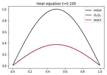
We compute the solution of the heat equation at \(t=0.1\). And, on the same graphic, we plot the initial condition, the exact solution and the numerical solution.
[7]:
import numpy as np
import sympy as sp
import pylab as plt
import pylbm

u, X, LA = sp.symbols('u, X, LA')

def solution(x, t):
    return np.sin(np.pi*x)*np.exp(-np.pi**2*mu*t)

xmin, xmax = 0., 1.
N = 128
mu = 1.
Tf = .1
dx = (xmax-xmin)/N # spatial step
la = 1./dx
s1 = 2./(1+2*mu)
s2 = 1.
dico = {
    'box':{'x': [xmin, xmax], 'label': 0},
    'space_step': dx,
    'scheme_velocity': la,
    'schemes': [
        {
            'velocities': list(range(3)),
            'conserved_moments': u,
            'polynomials': [1, X/LA, X**2/(2*LA**2)],
            'equilibrium': [u, 0., .5*u],
            'relaxation_parameters': [0., s1, s2],
        }
    ],
    'init': {u: (solution, (0.,))},
    'boundary_conditions': {
        0: {'method': {0: pylbm.bc.AntiBounceBack,}},
    },
    'parameters': {LA: la},
    'generator': 'numpy'
}

sol = pylbm.Simulation(dico)
x = sol.domain.x
y = sol.m[u]

plt.figure(1)
plt.plot(x, y, 'k', label='initial')

while sol.t < 0.1:
    sol.one_time_step()

plt.plot(x, sol.m[u], 'b', label=r'$D_1Q_3$')
plt.plot(x, solution(x, sol.t),'r', label='exact')
plt.title('Heat equation t={0:5.3f}'.format(sol.t))
plt.legend();