
With pylbm, the numerical simulations can be performed in a domain
with a complex geometry. This geometry is construct without considering a
particular mesh but only with geometrical objects.
All the geometrical informations are defined through a dictionary and
put into an object of the class Geometry.
News: it’s now possible to add a 3D geometrical object from a STL file.
First, the domain is put into a box: a segment in 1D, a rectangle in 2D, and a rectangular parallelepipoid in 3D.
Then, the domain is modified by adding or deleting some elementary shapes. In 2D, the elementary shapes are
From version 0.2, the geometrical elements are implemented in 3D, and from version 0.6, an element can be defined in a STL file. The elementary shapes are
Several examples of geometries can be found in demo/examples/geometry/
d = {"box": {"x": [0, 1], "label": [0, 1]}}
g = pylbm.Geometry(d)
g.visualize(viewlabel=True)
(Source code, png, pdf)
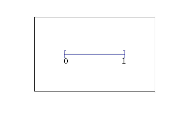
The segment \([0,1]\) is created by the dictionary with the key box.
We then add the labels 0 and 1 on the edges with the key label.
The result is then visualized with the labels by using the method
visualize.
If no labels are given in the dictionary, the default value is -1.
d = {"box": {"x": [0, 1], "y": [0, 1]}}
g = pylbm.Geometry(d)
g.visualize()
(Source code, png, pdf)
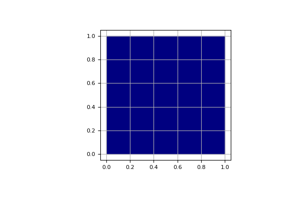
The square \([0,1]^2\) is created by the dictionary with the key box.
The result is then visualized by using the method
visualize.
We then add the labels on each edge of the square through a list of integers with the conventions:
|
|
d = {"box": {"x": [0, 1], "y": [0, 1], "label": [0, 1, 2, 3]}}
g = pylbm.Geometry(d)
g.visualize(viewlabel=True)
(Source code, png, pdf)
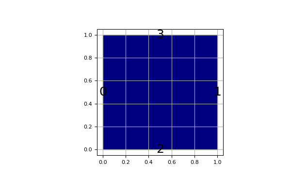
If all the labels have the same value, a shorter solution is to give only the integer value of the label instead of the list. If no labels are given in the dictionary, the default value is -1.
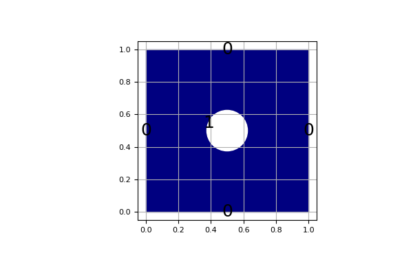
The unit square \([0,1]^2\) can be holed with a circle (script 1) or with a triangular or with a parallelogram (script 3)
In the first example,
a solid disc lies in the fluid domain defined by
a circle
with a center of (0.5, 0.5) and a radius of 0.125
d = {
    "box": {"x": [0, 1], "y": [0, 1], "label": 0},
    "elements": [pylbm.Circle((0.5, 0.5), 0.125, label=1)],
}
g = pylbm.Geometry(d)
g.visualize(viewlabel=True)
(Source code, png, pdf)

The dictionary of the geometry then contains an additional key elements
that is a list of elements.
In this example, the circle is labelized by 1 while the edges of the square by 0.
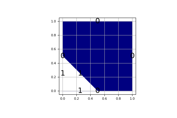
The element can be also a triangle
d = {
    "box": {"x": [0, 1], "y": [0, 1], "label": 0},
    "elements": [pylbm.Triangle((0.0, 0.0), (0.0, 0.5), (0.5, 0.0), label=1)],
}
g = pylbm.Geometry(d)
g.visualize(viewlabel=True)
(Source code, png, pdf)
or a parallelogram
d = {
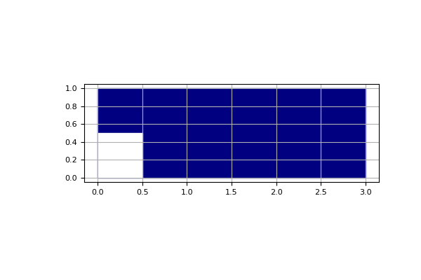
"box": {"x": [0, 3], "y": [0, 1], "label": [1, 2, 0, 0]},
"elements": [pylbm.Parallelogram((0.0, 0.0), (0.5, 0.0), (0.0, 0.5), label=0)],
}
g = pylbm.Geometry(d)
g.visualize()
(Source code, png, pdf)
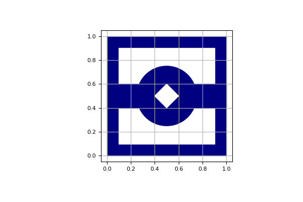
A complex geometry can be build by using a list of elements. In this example,
the box is fixed to the unit square \([0,1]^2\). A square hole is added with the
argument isfluid=False. A strip and a circle are then added with the argument
isfluid=True. Finally, a square hole is put. The value of elements
contains the list of all the previous elements. Note that the order of
the elements in the list is relevant.
square = pylbm.Parallelogram((0.1, 0.1), (0.8, 0), (0, 0.8), isfluid=False)
strip = pylbm.Parallelogram((0, 0.4), (1, 0), (0, 0.2), isfluid=True)
circle = pylbm.Circle((0.5, 0.5), 0.25, isfluid=True)
inner_square = pylbm.Parallelogram((0.4, 0.5), (0.1, 0.1), (0.1, -0.1), isfluid=False)
d = {
    "box": {"x": [0, 1], "y": [0, 1], "label": 0},
    "elements": [square, strip, circle, inner_square],
}
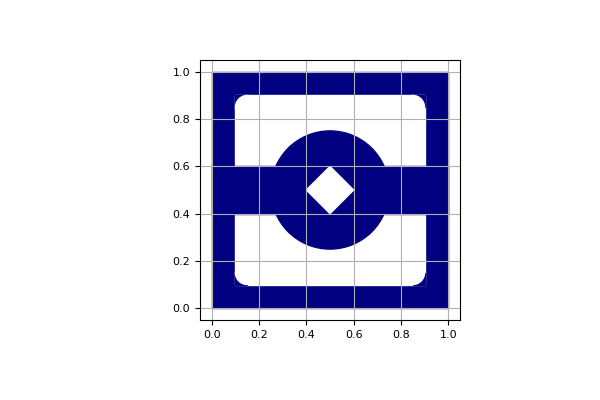
Once the geometry is built, it can be modified by adding or deleting other elements. For instance, the four corners of the cavity can be rounded in this way.
g.visualize()
# rounded inner angles
g.add_elem(pylbm.Parallelogram((0.1, 0.9), (0.05, 0), (0, -0.05), isfluid=True))
g.add_elem(pylbm.Circle((0.15, 0.85), 0.05, isfluid=False))
g.add_elem(pylbm.Parallelogram((0.1, 0.1), (0.05, 0), (0, 0.05), isfluid=True))
g.add_elem(pylbm.Circle((0.15, 0.15), 0.05, isfluid=False))
g.add_elem(pylbm.Parallelogram((0.9, 0.9), (-0.05, 0), (0, -0.05), isfluid=True))
g.add_elem(pylbm.Circle((0.85, 0.85), 0.05, isfluid=False))
g.add_elem(pylbm.Parallelogram((0.9, 0.1), (-0.05, 0), (0, 0.05), isfluid=True))
g.add_elem(pylbm.Circle((0.85, 0.15), 0.05, isfluid=False))
g.visualize()
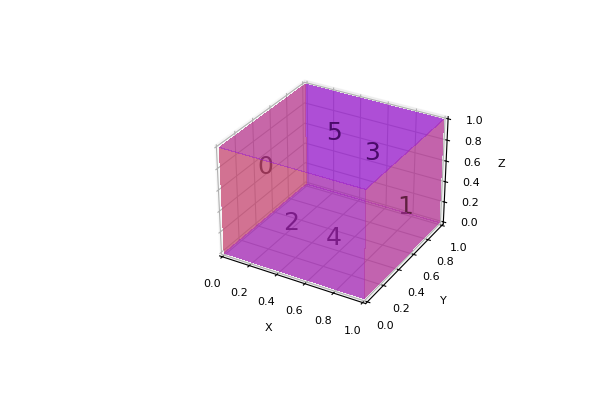
d = {"box": {"x": [0, 1], "y": [0, 1], "z": [0, 1], "label": list(range(6))}}
g = pylbm.Geometry(d)
g.visualize(viewlabel=True)
(Source code, png, pdf)

The cube \([0,1]^3\) is created by the dictionary with the key box.
The result is then visualized by using the method
visualize.
We then add the labels on each edge of the square through a list of integers with the conventions:
|
|
If all the labels have the same value, a shorter solution is to give only the integer value of the label instead of the list. If no labels are given in the dictionary, the default value is -1.
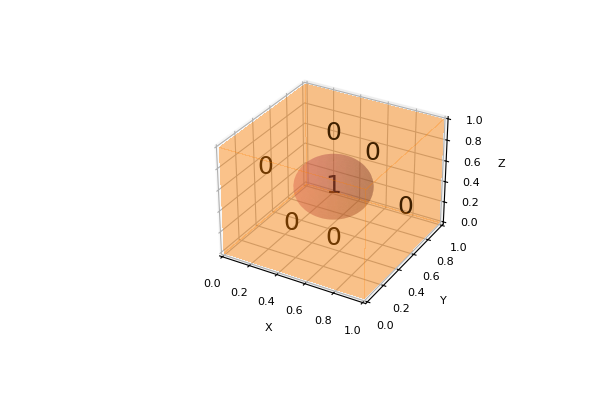
d = {
    "box": {"x": [0, 1], "y": [0, 1], "z": [0, 1], "label": 0},
    "elements": [pylbm.Sphere((0.5, 0.5, 0.5), 0.25, label=1)],
}
g = pylbm.Geometry(d)
g.visualize(viewlabel=True, alpha=0.25)
(Source code, png, pdf)

The cube \([0,1]^3\) and the spherical hole are created
by the dictionary with the keys box and elements.
The result is then visualized by using the method
visualize.
icosaedre = pylbm.STLElement("icosaedre.stl", label=1)
dico = {
    "box": {"x": [-3, 3], "y": [-3, 3], "z": [-3, 3], "label": 0},
    "elements": [icosaedre],
}
geom = pylbm.Geometry(dico)
print(geom)
geom.visualize(viewlabel=True, alpha=0.25)
(Source code, png, pdf)
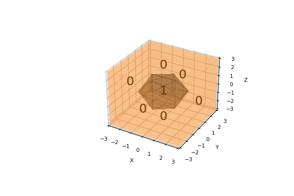
The icosaedre is created from a STL file and added in the geometry.
The result is then visualized by using the method
visualize.