In this tutorial, we test the most simple lattice Boltzmann scheme \(\DdQq{1}{2}\) on two classical hyperbolic scalar equations: the advection equation and the Burger’s equation.
## The advection equation
The problem reads
where \(c\) is a constant scalar (typically \(c=1\)). Additional boundary and initial conditions will be given in the following.
The numerical simulation of this equation by a lattice Boltzmann scheme consists in the approximation of the solution on discret points of \((0,1)\) at discret instants.
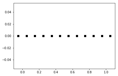
The spatial mesh is defined by using a numpy array. To simplify, the mesh is supposed to be uniform.
First, we import the package numpy and we create the spatial mesh. One phantom cell has to be added at each edge of the domain for the treatment of the boundary conditions.
[1]:
%matplotlib inline
[2]:
import numpy as np
import pylab as plt

def mesh(N):
    xmin, xmax = 0., 1.
    dx = 1./N
    x = np.linspace(xmin-.5*dx, xmax+.5*dx, N+2)
    return x

x = mesh(10)
plt.plot(x, 0.*x, 'sk')
plt.show()
To simulate this equation, we use the \(\DdQq{1}{2}\) scheme given by
two velocities \(v_0=-1\), \(v_1=1\), with associated distribution functions \(\fk{0}\) and \(\fk{1}\),
a space step \(\dx\) and a time step \(\dt\), the ration \(\lambda=\dx/\dt\) is called the scheme velocity,
two moments \(\mk{0}=\sum_{i=0}^1\fk{i}\) and \(\mk{1}=\lambda \sum_{i=0}^1 v_i\fk{i}\) and their equilibrium values \(\mke{0} = \mk{0}\), \(\mke{1} = c\mk{0}\),
a relaxation parameter \(s\) lying in \([0,2]\).
In order to prepare the formalism of the package pylbm, we introduce the two polynomials that define the moments: \(P_0 = 1\) and \(P_1=\lambda X\), such that
The transformation \((\fk{0}, \fk{1})\mapsto(\mk{0},\mk{1})\) is invertible if, and only if, the polynomials \((P_0,P_1)\) is a free set over the stencil of velocities.
The lattice Boltzmann method consists to compute the distribution functions \(\fk{0}\) and \(\fk{1}\) in each point of the lattice \(x\) and at each time \(t^n=n\dt\). A step of the scheme can be read as a splitting between the relaxation phase and the transport phase:
relaxation:
m2f:
transport:
f2m:
The moment of order \(0\), \(\mk{0}\), being the only one conserved during the relaxation phase, the equivalent equation of this scheme reads at first order
We implement a function equilibrium that computes the equilibrium value \(\mke{1}\), the moment of order \(0\), \(\mk{0}\), and the velocity \(c\) being given in argument.
[3]:
def equilibrium(m0, c):
    return c*m0
Then, we create two vectors \(\mk{0}\) and \(\mk{1}\) with shape the shape of the mesh and initialize them. The moment of order \(0\) should contain the initial value of the unknown \(u\) and the moment of order \(1\) the corresponding equilibrium value.
We create also two vectors \(\fk{0}\) and \(\fk{1}\).
[4]:
def initialize(mesh, c, la):
    m0 = np.zeros(mesh.shape)
    m0[np.logical_and(mesh<0.5, mesh>0.25)] = 1.
    m1 = equilibrium(m0, c)
    f0, f1 = np.empty(m0.shape), np.empty(m0.shape)
    m2f(f0, f1, m0, m1, la)
    return f0, f1, m0, m1
And finally, we implement the four elementary functions f2m, relaxation, m2f, and transport. In the transport function, the boundary conditions should be implemented: we will use periodic conditions by copying the informations in the phantom cells.
[5]:
def f2m(f0, f1, m0, m1, la):
    m0[:] = f0 + f1
    m1[:] = la*(f1 - f0)

def m2f(f0, f1, m0, m1, la):
    f0[:] = 0.5*(m0-m1/la)
    f1[:] = 0.5*(m0+m1/la)

def relaxation(m0, m1, c, s):
    m1[:] = (1-s)*m1 + s*equilibrium(m0, c)

def transport(f0, f1):
    #periodical boundary conditions
    f0[-1] = f0[1]
    f1[0] = f1[-2]
    #transport
    f0[1:-1] = f0[2:]
    f1[1:-1] = f1[:-2]
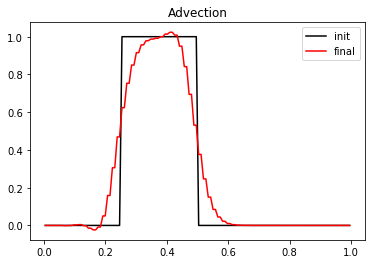
We compute and we plot the numerical solution at time \(T_f=2\).
[6]:
# parameters
c = .5  # velocity for the transport equation
Tf = 2. # final time
N = 128 # number of points in space
la = 1. # scheme velocity
s = 1.8 # relaxation parameter
# initialization
x = mesh(N)
f0, f1, m0, m1 = initialize(x, c, la)
t = 0
dt = (x[1]-x[0])/la
plt.figure(1)
plt.clf()
plt.plot(x[1:-1], m0[1:-1], 'k', label='init')
while t<Tf:
    t += dt
    relaxation(m0, m1, c, s)
    m2f(f0, f1, m0, m1, la)
    transport(f0, f1)
    f2m(f0, f1, m0, m1, la)
plt.plot(x[1:-1], m0[1:-1], 'r', label='final')
plt.legend()
plt.title('Advection')
plt.show()
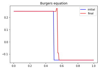
The problem reads
The previous \(\DdQq{1}{2}\) scheme can simulate the Burger’s equation by modifying the equilibrium value of the moment of order \(1\) \(\mke{1}\). It now reads \(\mke{1} = {\mk{0}}^2/2\).
More generaly, the simulated equation is into the conservative form
the equilibrium has to be taken to \(\mke{1}=\varphi(\mk{0})\).
We just have to modify the equilibrium and the initialization of the previous example to simulate the Burger’s equation. The initial condition can be a discontinuous function in order to simulate Riemann problems. Note that the function f2m, m2f, relaxation, and transport are unchanged.
[7]:
def equilibrium(m0):
    return .5*m0**2

def initialize(mesh, la):
    ug, ud = 0.25, -0.15
    xmin, xmax = .5*np.sum(mesh[:2]), .5*np.sum(mesh[-2:])
    xc = xmin + .5*(xmax-xmin)
    m0 = ug*(mesh<xc) + ud*(mesh>xc) + .5*(ug+ud)*(mesh==xc)
    m1 = equilibrium(m0)
    f0 = np.empty(m0.shape)
    f1 = np.empty(m0.shape)
    return f0, f1, m0, m1

def relaxation(m0, m1, s):
    m1[:] = (1-s)*m1 + s*equilibrium(m0)

# parameters
Tf = 1. # final time
N = 128 # number of points in space
la = 1. # scheme velocity
s = 1.8 # relaxation parameter
# initialization
x = mesh(N)     # mesh
dx = x[1]-x[0]  # space step
dt = dx/la      # time step
f0, f1, m0, m1 = initialize(x, la)
plt.figure(1)
plt.plot(x[1:-1], m0[1:-1], 'b', label='initial')
# time loops
t = 0.
while (t<Tf):
    t += dt
    relaxation(m0, m1, s)
    m2f(f0, f1, m0, m1, la)
    transport(f0, f1)
    f2m(f0, f1, m0, m1, la)
plt.plot(x[1:-1], m0[1:-1], 'r', label='final')
plt.title('Burgers equation')
plt.legend(loc='best')
plt.show()
We can test different values of the relaxation parameter \(s\). In particular, we observe that the scheme remains stable if \(s\in[0,2]\). More \(s\) is small, more the numerical diffusion is important and if \(s\) is close to \(2\), oscillations appear behind the shock.
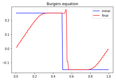
In order to simulate a Riemann problem, the boundary conditions have to be modified. A classical way is to impose entry conditions for hyperbolic problems. The lattice Boltzmann methods lend themselves very well to that conditions: the scheme only needs the distributions corresponding to a velocity that goes inside the domain. Nevertheless, on a physical edge where the flux is going outside, a non physical distribution that goes inside has to be imposed. A first simple way is to leave the initial value: this is correct while the discontinuity does not reach the edge. A second way is to impose Neumann condition by repeating the inner value.
We modify the previous script to take into account these new boundary conditions.
[8]:
def transport(f0, f1):
    # Neumann boundary conditions
    f0[-1] = f0[-2]
    f1[0] = f1[1]
    # transport
    f0[1:-1] = f0[2:]
    f1[1:-1] = f1[:-2]

# parameters
Tf = 1. # final time
N = 128 # number of points in space
la = 1. # scheme velocity
s = 1.8 # relaxation parameter

# initialization
x = mesh(N)     # mesh
dx = x[1]-x[0]  # space step
dt = dx/la      # time step
f0, f1, m0, m1 = initialize(x, la)
plt.figure(1)
plt.plot(x[1:-1], m0[1:-1], 'b', label='initial')
# time loops
t = 0.
while (t<Tf):
    t += dt
    relaxation(m0, m1, s)
    m2f(f0, f1, m0, m1, la)
    transport(f0, f1)
    f2m(f0, f1, m0, m1, la)
plt.plot(x[1:-1], m0[1:-1], 'r', label='final')
plt.title('Burgers equation')
plt.legend(loc='best')
plt.show()