The wave equation in 1D¶

The scheme \(\DdQq{1}{3}\)¶

The numerical simulation of this equation by a lattice Boltzmann scheme consists in the approximation of the solution on discret points of \((0,2\pi)\) at discret instants.

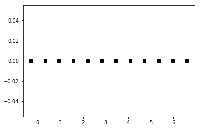
The spatial mesh is defined by using a numpy array. To simplify, the mesh is supposed to be uniform.

First, we import the package numpy and we create the spatial mesh. One phantom cell has to be added at each bound for the treatment of the boundary conditions.

[1]:

%matplotlib inline

[2]:

import numpy as np
import pylab as plt

def mesh(N):
    xmin, xmax = 0., 2.*np.pi
    dx = (xmax-xmin)/N
    x = np.linspace(xmin-.5*dx, xmax+.5*dx, N+2)
    return x

x = mesh(10)
plt.plot(x, 0.*x, 'sk')
plt.show()

To simulate this system of equations, we use the \(\DdQq{1}{3}\) scheme given by

• three velocities \(v_0=0\), \(v_1=1\), and \(v_2=-1\), with associated distribution functions \(\fk{0}\), \(\fk{1}\), and \(\fk{2}\),

• a space step \(\dx\) and a time step \(\dt\), the ration \(\lambda=\dx/\dt\) is called the scheme velocity,

• three moments

  \[\mk{0}=\sum_{i=0}^{2} \fk{i}, \quad \mk{1}= \lambda \sum_{i=0}^{2} v_i \fk{i}, \quad \mk{2}= \frac{\lambda^2}{2} \sum_{i=0}^{2} v_i^2 \fk{i},\]

and their equilibrium values \(\mke{0} = \mk{0}\), \(\mke{1} = \mk{1}\), and \(\mke{2} = c^2/2 \mk{0}\).

• a relaxation parameter \(s\) lying in \([0,2]\).

In order to prepare the formalism of the package pylbm, we introduce the three polynomials that define the moments: \(P_0 = 1\), \(P_1=\lambda X\), and \(P_2=\lambda^2/2 X^2\), such that

The transformation \((\fk{0}, \fk{1}, \fk{2})\mapsto(\mk{0},\mk{1}, \mk{2})\) is invertible if, and only if, the polynomials \((P_0,P_1,P_2)\) is a free set over the stencil of velocities.

The lattice Boltzmann method consists to compute the distribution functions \(\fk{0}\), \(\fk{1}\), and \(\fk{2}\) in each point of the lattice \(x\) and at each time \(t^n=n\dt\). A step of the scheme can be read as a splitting between the relaxation phase and the transport phase:

• relaxation:

  \[\mks{2}(t,x)=(1-s)\mk{2}(t,x)+s\mke{2}(t,x).\]

• m2f:

  \[\begin{split}\begin{aligned}\fks{0}(t,x)&\;=\mk{0}(t,x)-2\mks{2}(t,x)/\lambda^2, \\ \fks{1}(t,x)&\;=\mk{1}(t,x)/(2\lambda)+\mks{2}(t,x)/\lambda^2, \\ \fks{2}(t,x)&\;=-\mk{1}(t,x)/(2\lambda)+\mks{2}(t,x)/\lambda^2.\end{aligned}\end{split}\]

• transport:

  \[\begin{split}\begin{aligned} \fk{0}(t+\dt, x)&\;=\fks{0}(t,x), \\ \fk{1}(t+\dt, x)&\;=\fks{1}(t,x-\dx), \\ \fk{2}(t+\dt, x)&\;=\fks{2}(t,x+\dx). \end{aligned}\end{split}\]

• f2m:

  \[\begin{split}\begin{aligned}\mk{0}(t+\dt,x)&\;=\fk{0}(t+\dt,x)+\fk{1}(t+\dt,x)+\fk{2}(t+\dt,x), \\ \mk{1}(t+\dt,x)&\;=\lambda\fk{1}(t+\dt,x)-\lambda\fk{2}(t+\dt,x), \\ \mk{2}(t+\dt,x)&\;=\tfrac{1}{2}\lambda^2\fk{1}(t+\dt,x)+\tfrac{1}{2}\lambda^2\fk{2}(t+\dt,x).\end{aligned}\end{split}\]

The moments of order \(0\), \(\mk{0}\), and of order \(1\), \(\mk{1}\), being conserved during the relaxation phase, the equivalent equations of this scheme read at first order

We implement a function equilibrium that computes the equilibrium value \(\mke{2}\), the moment of order \(0\), \(\mk{0}\), and the velocity \(c\) being given in argument.

[3]:

def equilibrium(m0, c):
    return .5*c**2*m0

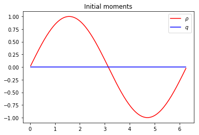
We create three vectors \(\mk{0}\), \(\mk{1}\), and \(\mk{2}\) with shape the shape of the mesh and initialize them. The moments of order \(0\) and \(1\) should contain the initial value of the unknowns \(\rho\) and \(q\), and the moment of order \(2\) the corresponding equilibrium value.

We create also three vectors \(\fk{0}\), \(\fk{1}\) and \(\fk{2}\).

[4]:

def initialize(mesh, c, la):
    m0 = np.sin(mesh)
    m1 = np.zeros(mesh.shape)
    m2 = equilibrium(m0, c)
    f0 = np.empty(m0.shape)
    f1 = np.empty(m0.shape)
    f2 = np.empty(m0.shape)
    return f0, f1, f2, m0, m1, m2

## Periodic boundary conditions

We implement the four elementary functions f2m, relaxation, m2f, and transport. In the transport function, the boundary conditions should be implemented: we will use periodic conditions by copying the informations in the phantom cells.

[5]:

def f2m(f0, f1, f2, m0, m1, m2, la):
    m0[:] = f0 + f1 + f2
    m1[:] = la * (f2 - f1)
    m2[:] = .5* la**2 * (f1 + f2)

def m2f(f0, f1, f2, m0, m1, m2, la):
    f0[:] = m0 - 2./la**2 * m2
    f1[:] = -.5/la * m1 + 1/la**2 * m2
    f2[:] = .5/la * m1 + 1/la**2 * m2

def relaxation(m0, m1, m2, c, s):
    m2[:] *= (1-s)
    m2[:] += s*equilibrium(m0, c)

def transport(f0, f1, f2):
    # periodic boundary conditions
    f1[-1] = f1[1]
    f2[0] = f2[-2]
    # transport
    f1[1:-1] = f1[2:]
    f2[1:-1] = f2[:-2]

We compute and we plot the numerical solution at time \(T_f=2\pi\).

[6]:

# parameters
c = 1   # velocity for the transport equation
Tf = 2.*np.pi # final time
N = 128 # number of points in space
la = 1. # scheme velocity
s = 2.  # relaxation parameter
# initialization
x = mesh(N)     # mesh
dx = x[1]-x[0]  # space step
dt = dx/la      # time step
f0, f1, f2, m0, m1, m2 = initialize(x, c, la)
plt.figure(1)
plt.plot(x[1:-1], m0[1:-1], 'r', label=r'$\rho$')
plt.plot(x[1:-1], m1[1:-1], 'b', label=r'$q$')
plt.title('Initial moments')
plt.legend(loc='best')
# time loops
nt = int(Tf/dt)
m2f(f0, f1, f2, m0, m1, m2, la)
for k in range(nt):
    transport(f0, f1, f2)
    f2m(f0, f1, f2, m0, m1, m2, la)
    relaxation(m0, m1, m2, c, s)
    m2f(f0, f1, f2, m0, m1, m2, la)
plt.figure(2)
plt.plot(x[1:-1], m0[1:-1], 'r', label=r'$\rho$')
plt.plot(x[1:-1], m1[1:-1], 'b', label=r'$q$')
plt.title('Final moments')
plt.legend(loc='best')
plt.show()

Anti bounce back conditions¶

In order to take into account homogenous Dirichlet conditions over \(\rho\), we introduce the bounce back conditions. At edge \(x=0\), two points are involved: \(x_0=-\dx/2\) and \(x_1=\dx/2\). We impose \(\fk{1}(x_0)=-\fk{2}(x_1)\). And at edge \(x=2\pi\), the two involved points are \(x_{N}\) and \(x_{N+1}\). We impose \(\fk{2}(x_{N+1})=-\fk{1}(x_{N})\).

We modify the transport function to impose anti bounce back conditions. We can compare the solutions obtained with the two different boundary conditions.

[7]:

def transport(f0, f1, f2):
    # anti bounce back boundary conditions
    f1[-1] = -f2[-2]
    f2[0] = -f1[1]
    # transport
    f1[1:-1] = f1[2:]
    f2[1:-1] = f2[:-2]


# parameters
c = 1   # velocity for the transport equation
Tf = 2*np.pi # final time
N = 128 # number of points in space
la = 1. # scheme velocity
s = 2.  # relaxation parameter
# initialization
x = mesh(N)     # mesh
dx = x[1]-x[0]  # space step
dt = dx/la      # time step
f0, f1, f2, m0, m1, m2 = initialize(x, c, la)
plt.figure(1)
plt.plot(x[1:-1], m0[1:-1], 'r', label=r'$\rho$')
plt.plot(x[1:-1], m1[1:-1], 'b', label=r'$q$')
plt.title('Initial moments')
plt.legend(loc='best')
# time loops
nt = int(Tf/dt)
m2f(f0, f1, f2, m0, m1, m2, la)
for k in range(nt):
    transport(f0, f1, f2)
    f2m(f0, f1, f2, m0, m1, m2, la)
    relaxation(m0, m1, m2, c, s)
    m2f(f0, f1, f2, m0, m1, m2, la)
plt.figure(2)
plt.plot(x[1:-1], m0[1:-1], 'r', label=r'$\rho$')
plt.plot(x[1:-1], m1[1:-1], 'b', label=r'$q$')
plt.title('Final moments')
plt.legend(loc='best')
plt.show()

[ ]: