[1]:
%matplotlib inline
In this tutorial, we test a very classical lattice Boltzmann scheme \(\DdQq{2}{5}\) on the heat equation.
The problem reads
where \(\mu\) is a constant scalar.
The numerical simulation of this equation by a lattice Boltzmann scheme consists in the approximatation of the solution on discret points of \((0,1)^2\) at discret instants.
To simulate this system of equations, we use the \(\DdQq{2}{5}\) scheme given by
five velocities \(v_0=(0,0)\), \(v_1=(1,0)\), \(v_2=(0,1)\), \(v_3=(-1,0)\), and \(v_4=(0,-1)\) with associated distribution functions \(\fk{i}\), \(0\leq i\leq 4\),
a space step \(\dx\) and a time step \(\dt\), the ration \(\lambda=\dx/\dt\) is called the scheme velocity,
five moments
and their equilibrium values \(\mke{k}\), \(0\leq k\leq 4\).
two relaxation parameters \(s_1\) and \(s_2\) lying in \([0,2]\) (\(s_1\) for the odd moments and \(s_2\) for the odd ones).
In order to use the formalism of the package pylbm, we introduce the five polynomials that define the moments: \(P_0 = 1\), \(P_1=X\), \(P_2=Y\), \(P_3=(X^2+Y^2)/2\), and \(P_4=(X^2-Y^2)/2\), such that
The transformation \((\fk{0}, \fk{1}, \fk{2}, \fk{3}, \fk{4})\mapsto(\mk{0},\mk{1}, \mk{2}, \mk{3}, \mk{4})\) is invertible if, and only if, the polynomials \((P_0,P_1,P_2,P_3,P_4)\) is a free set over the stencil of velocities.
The lattice Boltzmann method consists to compute the distribution functions \(\fk{i}\), \(0\leq i\leq 4\) in each point of the lattice \(x\) and at each time \(t^n=n\dt\). A step of the scheme can be read as a splitting between the relaxation phase and the transport phase:
relaxation:
m2f:
transport:
f2m:
The moment of order \(0\), \(\mk{0}\), being conserved during the relaxation phase, a diffusive scaling \(\dt=\dx^2\), yields to the following equivalent equation
if \(\mke{1}=0\). In order to be consistent with the heat equation, the following choice is done:
pylbm uses Python dictionary to describe the simulation. In the following, we will build this dictionary step by step.
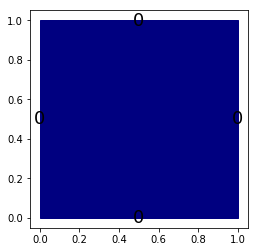
In pylbm, the geometry is defined by a box and a label for the boundaries. We define here a square \((0, 1)^2\).
[2]:
import pylbm
import numpy as np
import pylab as plt
xmin, xmax, ymin, ymax = 0., 1., 0., 1.
dico_geom = {
    'box': {'x': [xmin, xmax],
            'y': [ymin, ymax],
            'label': 0
           },
}
geom = pylbm.Geometry(dico_geom)
print(geom)
geom.visualize(viewlabel=True);
+----------------------+
| Geometry information |
+----------------------+
    - spatial dimension: 2
    - bounds of the box: [0. 1.] x [0. 1.]
    - labels: [0, 0, 0, 0]
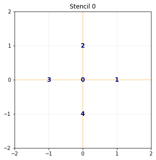
pylbm provides a class stencil that is used to define the discret velocities of the scheme. In this example, the stencil is composed by the velocities \(v_0=(0,0)\), \(v_1=(1,0)\), \(v_2=(-1,0)\), \(v_3=(0,1)\), and \(v_4=(0,-1)\) numbered by \([0,1,2,3,4]\).
[3]:
dico_sten = {
    'dim':2,
    'schemes': [
        {'velocities': list(range(5))}
    ],
}
sten = pylbm.Stencil(dico_sten)
print(sten)
sten.visualize();
+---------------------+
| Stencil information |
+---------------------+
    - spatial dimension: 2
    - minimal velocity in each direction: [-1 -1]
    - maximal velocity in each direction: [1 1]
    - information for each elementary stencil:
        stencil 0
            - number of velocities: 5
            - velocities
                (0: 0, 0)
                (1: 1, 0)
                (2: 0, 1)
                (3: -1, 0)
                (4: 0, -1)
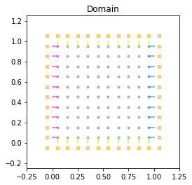
### The domain
In order to build the domain of the simulation, the dictionary should contain the space step \(\dx\) and the stencils of the velocities (one for each scheme).
We construct a domain with \(N=10\) points in space.
[4]:
N = 10
dx = (xmax-xmin)/N
dico_dom = {
    'box': {'x': [xmin, xmax],
            'y': [ymin, ymax],
            'label': 0
           },
    'space_step': dx,
    'schemes': [
        {'velocities': list(range(5)),}
    ],
}
dom = pylbm.Domain(dico_dom)
print(dom)
dom.visualize(view_distance=True);
+--------------------+
| Domain information |
+--------------------+
    - spatial dimension: 2
    - space step: 0.1
    - with halo:
        bounds of the box: [-0.05 -0.05] x [1.05 1.05]
        number of points: [12, 12]
    - without halo:
        bounds of the box: [0.05 0.05] x [0.95 0.95]
        number of points: [10, 10]

    +----------------------+
    | Geometry information |
    +----------------------+
        - spatial dimension: 2
        - bounds of the box: [0. 1.] x [0. 1.]
        - labels: [0, 0, 0, 0]
In pylbm, a simulation can be performed by using several coupled schemes. In this example, a single scheme is used and defined through a list of one single dictionary. This dictionary should contain:
‘velocities’: a list of the velocities
‘conserved_moments’: a list of the conserved moments as sympy variables
‘polynomials’: a list of the polynomials that define the moments
‘equilibrium’: a list of the equilibrium value of all the moments
‘relaxation_parameters’: a list of the relaxation parameters (\(0\) for the conserved moments)
‘init’: a dictionary to initialize the conserved moments
(see the documentation for more details)
The scheme velocity could be taken to \(1/\dx\) and the inital value of \(u\) to
[5]:
import sympy as sp

def solution(x, y, t):
    return np.sin(np.pi*x)*np.sin(np.pi*y)*np.exp(-2*np.pi**2*mu*t)

# parameters
mu = 1.
la = 1./dx
s1 = 2./(1+4*mu)
s2 = 1.
u, X, Y, LA = sp.symbols('u, X, Y, LA')

dico_sch = {
    'dim': 2,
    'scheme_velocity': la,
    'schemes': [
        {
            'velocities': list(range(5)),
            'conserved_moments': u,
            'polynomials': [1, X/LA, Y/LA, (X**2+Y**2)/(2*LA**2), (X**2-Y**2)/(2*LA**2)],
            'equilibrium': [u, 0., 0., .5*u, 0.],
            'relaxation_parameters': [0., s1, s1, s2, s2],
        }
    ],
    'parameters': {LA: la},
}

sch = pylbm.Scheme(dico_sch)
print(sch)
+--------------------+
| Scheme information |
+--------------------+
    - spatial dimension: 2
    - number of schemes: 1
    - number of velocities: 5
    - conserved moments: [u]

    +----------+
    | Scheme 0 |
    +----------+
        - velocities
            (0: 0, 0)
            (1: 1, 0)
            (2: 0, 1)
            (3: -1, 0)
            (4: 0, -1)

        - polynomials

            ⎡   1   ⎤
            ⎢       ⎥
            ⎢  X    ⎥
            ⎢  ──   ⎥
            ⎢  LA   ⎥
            ⎢       ⎥
            ⎢  Y    ⎥
            ⎢  ──   ⎥
            ⎢  LA   ⎥
            ⎢       ⎥
            ⎢ 2    2⎥
            ⎢X  + Y ⎥
            ⎢───────⎥
            ⎢     2 ⎥
            ⎢ 2⋅LA  ⎥
            ⎢       ⎥
            ⎢ 2    2⎥
            ⎢X  - Y ⎥
            ⎢───────⎥
            ⎢     2 ⎥
            ⎣ 2⋅LA  ⎦

        - equilibria

            ⎡  u  ⎤
            ⎢     ⎥
            ⎢ 0.0 ⎥
            ⎢     ⎥
            ⎢ 0.0 ⎥
            ⎢     ⎥
            ⎢0.5⋅u⎥
            ⎢     ⎥
            ⎣ 0.0 ⎦

        - relaxation parameters

            ⎡0.0⎤
            ⎢   ⎥
            ⎢0.4⎥
            ⎢   ⎥
            ⎢0.4⎥
            ⎢   ⎥
            ⎢1.0⎥
            ⎢   ⎥
            ⎣1.0⎦

    - moments matrices

        ⎡1   1    1     1     1  ⎤
        ⎢                        ⎥
        ⎢   10         -10       ⎥
        ⎢0  ──    0    ────   0  ⎥
        ⎢   LA          LA       ⎥
        ⎢                        ⎥
        ⎢         10         -10 ⎥
        ⎢0   0    ──    0    ────⎥
        ⎢         LA          LA ⎥
        ⎢                        ⎥
        ⎢    50   50    50    50 ⎥
        ⎢0  ───  ───   ───   ─── ⎥
        ⎢     2    2     2     2 ⎥
        ⎢   LA   LA    LA    LA  ⎥
        ⎢                        ⎥
        ⎢    50  -50    50   -50 ⎥
        ⎢0  ───  ────  ───   ────⎥
        ⎢     2    2     2     2 ⎥
        ⎣   LA   LA    LA    LA  ⎦

    - inverse of moments matrices

        ⎡                  2        ⎤
        ⎢               -LA         ⎥
        ⎢1   0     0    ─────    0  ⎥
        ⎢                 50        ⎥
        ⎢                           ⎥
        ⎢                  2      2 ⎥
        ⎢    LA          LA     LA  ⎥
        ⎢0   ──    0     ───    ─── ⎥
        ⎢    20          200    200 ⎥
        ⎢                           ⎥
        ⎢                  2      2 ⎥
        ⎢          LA    LA    -LA  ⎥
        ⎢0   0     ──    ───   ─────⎥
        ⎢          20    200    200 ⎥
        ⎢                           ⎥
        ⎢                  2      2 ⎥
        ⎢   -LA          LA     LA  ⎥
        ⎢0  ────   0     ───    ─── ⎥
        ⎢    20          200    200 ⎥
        ⎢                           ⎥
        ⎢                  2      2 ⎥
        ⎢         -LA    LA    -LA  ⎥
        ⎢0   0    ────   ───   ─────⎥
        ⎣          20    200    200 ⎦
A simulation is built by defining a correct dictionary.
We combine the previous dictionaries to build a simulation. In order to impose the homogeneous Dirichlet conditions in \(x=0\), \(x=1\), \(y=0\), and \(y=1\), the dictionary should contain the key ‘boundary_conditions’ (we use pylbm.bc.Anti_bounce_back function).
[6]:
dico = {
    'box': {'x': [xmin, xmax],
            'y': [ymin, ymax],
            'label': 0},
    'space_step': dx,
    'scheme_velocity': la,
    'schemes': [
        {
            'velocities': list(range(5)),
            'conserved_moments': u,
            'polynomials': [1, X/LA, Y/LA, (X**2+Y**2)/(2*LA**2), (X**2-Y**2)/(2*LA**2)],
            'equilibrium': [u, 0., 0., .5*u, 0.],
            'relaxation_parameters': [0., s1, s1, s2, s2],
        }
    ],
    'init': {u: (solution, (0.,))},
    'boundary_conditions': {
        0: {'method': {0: pylbm.bc.AntiBounceBack,}},
    },
    'parameters': {LA: la},
}

sol = pylbm.Simulation(dico)
print(sol)
+------------------------+
| Simulation information |
+------------------------+

    +--------------------+
    | Domain information |
    +--------------------+
        - spatial dimension: 2
        - space step: 0.1
        - with halo:
            bounds of the box: [-0.05 -0.05] x [1.05 1.05]
            number of points: [12, 12]
        - without halo:
            bounds of the box: [0.05 0.05] x [0.95 0.95]
            number of points: [10, 10]

        +----------------------+
        | Geometry information |
        +----------------------+
            - spatial dimension: 2
            - bounds of the box: [0. 1.] x [0. 1.]
            - labels: [0, 0, 0, 0]

    +--------------------+
    | Scheme information |
    +--------------------+
        - spatial dimension: 2
        - number of schemes: 1
        - number of velocities: 5
        - conserved moments: [u]

        +----------+
        | Scheme 0 |
        +----------+
            - velocities
                (0: 0, 0)
                (1: 1, 0)
                (2: 0, 1)
                (3: -1, 0)
                (4: 0, -1)

            - polynomials

                ⎡   1   ⎤
                ⎢       ⎥
                ⎢  X    ⎥
                ⎢  ──   ⎥
                ⎢  LA   ⎥
                ⎢       ⎥
                ⎢  Y    ⎥
                ⎢  ──   ⎥
                ⎢  LA   ⎥
                ⎢       ⎥
                ⎢ 2    2⎥
                ⎢X  + Y ⎥
                ⎢───────⎥
                ⎢     2 ⎥
                ⎢ 2⋅LA  ⎥
                ⎢       ⎥
                ⎢ 2    2⎥
                ⎢X  - Y ⎥
                ⎢───────⎥
                ⎢     2 ⎥
                ⎣ 2⋅LA  ⎦

            - equilibria

                ⎡  u  ⎤
                ⎢     ⎥
                ⎢ 0.0 ⎥
                ⎢     ⎥
                ⎢ 0.0 ⎥
                ⎢     ⎥
                ⎢0.5⋅u⎥
                ⎢     ⎥
                ⎣ 0.0 ⎦

            - relaxation parameters

                ⎡0.0⎤
                ⎢   ⎥
                ⎢0.4⎥
                ⎢   ⎥
                ⎢0.4⎥
                ⎢   ⎥
                ⎢1.0⎥
                ⎢   ⎥
                ⎣1.0⎦

        - moments matrices

            ⎡1   1    1     1     1  ⎤
            ⎢                        ⎥
            ⎢   10         -10       ⎥
            ⎢0  ──    0    ────   0  ⎥
            ⎢   LA          LA       ⎥
            ⎢                        ⎥
            ⎢         10         -10 ⎥
            ⎢0   0    ──    0    ────⎥
            ⎢         LA          LA ⎥
            ⎢                        ⎥
            ⎢    50   50    50    50 ⎥
            ⎢0  ───  ───   ───   ─── ⎥
            ⎢     2    2     2     2 ⎥
            ⎢   LA   LA    LA    LA  ⎥
            ⎢                        ⎥
            ⎢    50  -50    50   -50 ⎥
            ⎢0  ───  ────  ───   ────⎥
            ⎢     2    2     2     2 ⎥
            ⎣   LA   LA    LA    LA  ⎦

        - inverse of moments matrices

            ⎡                  2        ⎤
            ⎢               -LA         ⎥
            ⎢1   0     0    ─────    0  ⎥
            ⎢                 50        ⎥
            ⎢                           ⎥
            ⎢                  2      2 ⎥
            ⎢    LA          LA     LA  ⎥
            ⎢0   ──    0     ───    ─── ⎥
            ⎢    20          200    200 ⎥
            ⎢                           ⎥
            ⎢                  2      2 ⎥
            ⎢          LA    LA    -LA  ⎥
            ⎢0   0     ──    ───   ─────⎥
            ⎢          20    200    200 ⎥
            ⎢                           ⎥
            ⎢                  2      2 ⎥
            ⎢   -LA          LA     LA  ⎥
            ⎢0  ────   0     ───    ─── ⎥
            ⎢    20          200    200 ⎥
            ⎢                           ⎥
            ⎢                  2      2 ⎥
            ⎢         -LA    LA    -LA  ⎥
            ⎢0   0    ────   ───   ─────⎥
            ⎣          20    200    200 ⎦
Once the simulation is initialized, one time step can be performed by using the function one_time_step.
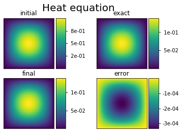
We compute the solution of the heat equation at \(t=0.1\). On the same graphic, we plot the initial condition, the exact solution and the numerical solution.
[7]:
import numpy as np
import sympy as sp
import pylab as plt
%matplotlib inline
from mpl_toolkits.axes_grid1 import make_axes_locatable
import pylbm

u, X, Y = sp.symbols('u, X, Y')

def solution(x, y, t, k, l):
    return np.sin(k*np.pi*x)*np.sin(l*np.pi*y)*np.exp(-(k**2+l**2)*np.pi**2*mu*t)

def plot(i, j, z, title):
    im = axarr[i,j].imshow(z)
    divider = make_axes_locatable(axarr[i, j])
    cax = divider.append_axes("right", size="20%", pad=0.05)
    cbar = plt.colorbar(im, cax=cax, format='%6.0e')
    axarr[i, j].xaxis.set_visible(False)
    axarr[i, j].yaxis.set_visible(False)
    axarr[i, j].set_title(title)

# parameters
xmin, xmax, ymin, ymax = 0., 1., 0., 1.
N = 128
mu = 1.
Tf = .1
dx = (xmax-xmin)/N # spatial step
la = 1./dx
s1 = 2./(1+4*mu)
s2 = 1.
k, l = 1, 1 # number of the wave

dico = {
    'box': {'x':[xmin, xmax],
            'y':[ymin, ymax],
            'label': 0},
    'space_step': dx,
    'scheme_velocity': la,
    'schemes':[
        {
            'velocities': list(range(5)),
            'conserved_moments': u,
            'polynomials': [1, X/LA, Y/LA, (X**2+Y**2)/(2*LA**2), (X**2-Y**2)/(2*LA**2)],
            'equilibrium': [u, 0., 0., .5*u, 0.],
            'relaxation_parameters': [0., s1, s1, s2, s2],
        }
    ],
    'init': {u: (solution, (0., k, l))},
    'boundary_conditions': {
        0: {'method': {0: pylbm.bc.AntiBounceBack,}},
    },
    'generator': 'cython',
    'parameters': {LA: la},
}

sol = pylbm.Simulation(dico)
x = sol.domain.x
y = sol.domain.y

f, axarr = plt.subplots(2, 2)
f.suptitle('Heat equation', fontsize=20)

plot(0, 0, sol.m[u].copy(), 'initial')

while sol.t < Tf:
    sol.one_time_step()

sol.f2m()
z = sol.m[u]
ze = solution(x[:, np.newaxis], y[np.newaxis, :], sol.t, k, l)
plot(1, 0, z, 'final')
plot(0, 1, ze, 'exact')
plot(1, 1, z-ze, 'error')

plt.show()